Chaos and Fractals

Subsection 6.1.1 Definition of self-affinity

Let's start with a simple example, as shown in Figure 6.1.1.

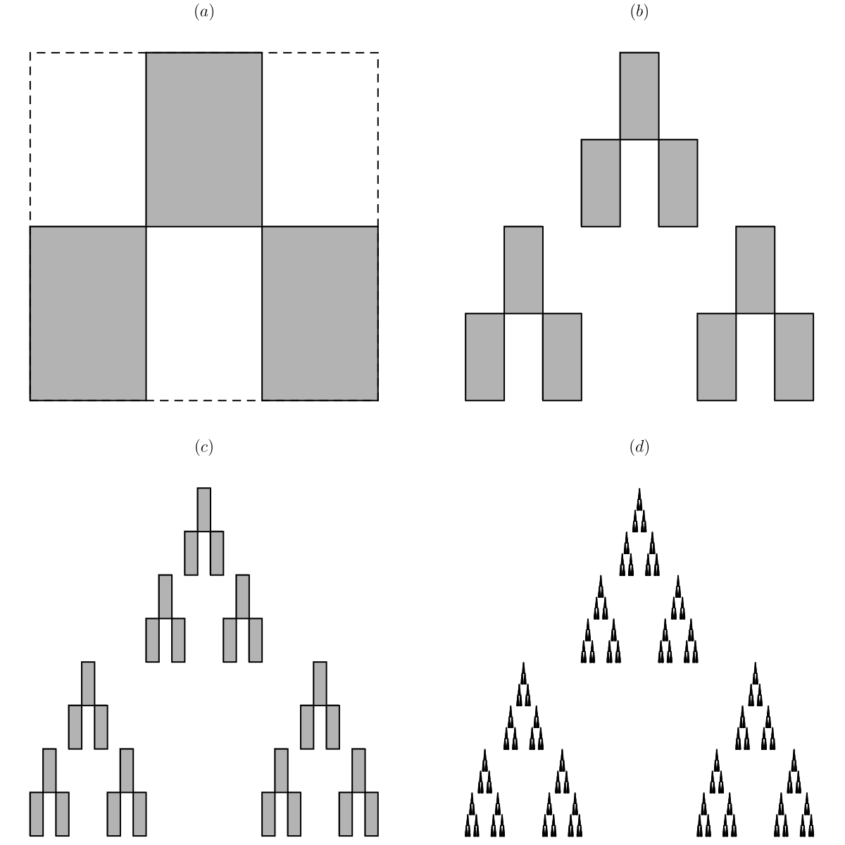
Figure 6.1.1 (a) portrays the action of an IFS of three similarities on the unit square. The dashed outline of the unit square contains the three shaded images of the square under the action of the IFS. Figures Figure 6.1.1 (b) and Figure 6.1.1 (c) show the second and third level approximations and Figure 6.1.1 (d) is a higher level approximation. Note that the key difference between a similarity and an affine function is that an affine functions may contract by different amounts in different directions. Thus the images of the square may be rectangles, or even parallelograms. In this particular example, the set is generated by the IFS

where

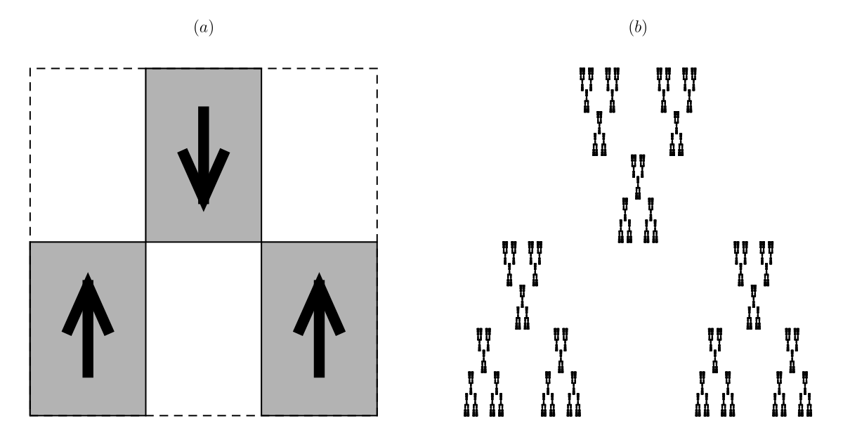
Of course, affine transformations can rotate and/or reflect an object as well. Figure 6.1.2 illustrates a self-affine set where reflection is used for one of the transformations. As before, Figure 6.1.2 (a) portrays the action of an IFS of three similarities on the unit square; this time, however, the initial square has an upward orientation. The image shows how one of the rectangles has been flipped using the matrix

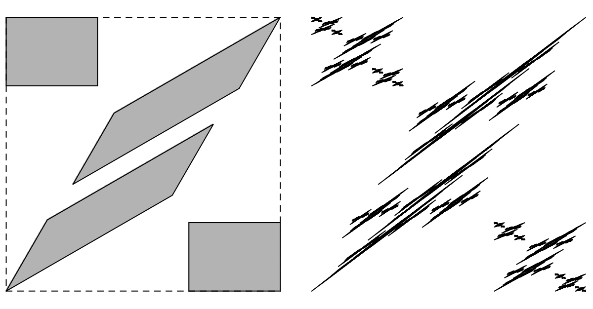
Affine functions can also have a shear effect, which a similarity cannot. Figure 6.1.3 shows such a set constructed with four affine transformations, two of which involve a shear. The two matrices used in the generation of this set are

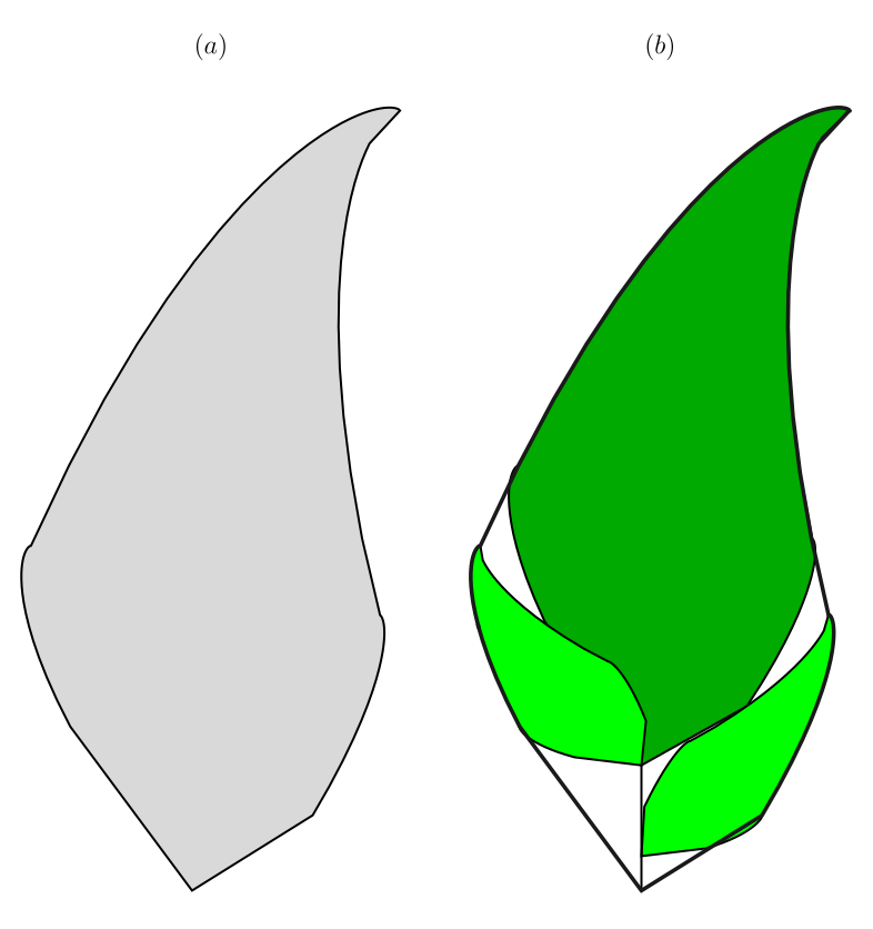
Our last example, Barnsley’s Fern, is shown in Figure 6.1.4 and is truly incredible. The obvious difference between Barnsley’s fern and our other examples is its natural appearance. The amazing thing is that it is generated using an IFS with only four affine functions. Since an affine function is specified by six numbers, this means that only 24 numbers are required to encode this very natural looking object.

Barnsley’s fern is the invariant set of the following IFS.

Figure 6.1.5 shows the action of the IFS on an outline of the fern. Note that the function \(f_4\) maps all of \(\mathbb{R}^2\) onto the \(y\)-axis. In particular, \(f_4\) maps the entire fern onto the stem at the bottom of Figure 6.1.5 (b).

Subsection 6.1.2 Tools

Both of the tools we used for self-similar sets can deal with self-affine sets as well. You can read more in this Observable notebook.

Subsection 6.1.3 The Collage Theorem

Barnsley’s fern suggests that we might be able to use iterated function systems to approximate natural images. To do so, we would like a method to find an iterated function system whose invariant set is close to a given set. The theoretical tool for doing this is called the collage theorem.

In other words, if an IFS doesn’t move a particular compact set \(F\) too much and the IFS has small contraction ratios, then the set \(F\) must be close to the attractor of the IFS. Now suppose we have a compact set \(A\) that we would like to approximate with an IFS. We should attempt to find a compact set \(F\) which is close to \(A\) and an IFS with small contraction ratios which moves \(F\) very little in the Hausdorff metric. Then the collage theorem guarantees that the invariant set \(E\) of the IFS will be close to \(F\text{.}\) Since \(F\) is close to \(A\text{,}\) \(E\) will be close to \(A\text{.}\)

As an example, suppose we would like an IFS whose invariant set is approximately the closed unit disk. Although this is not a very natural looking target set, the example is interesting since the disk is manifestly not self-similar. We first find a collection of small disks whose union is close to the unit disk in the Hausdorff metric. Such a collection of disks is shown in Figure 6.1.7 (a) which also shows the boundary of the unit disk.

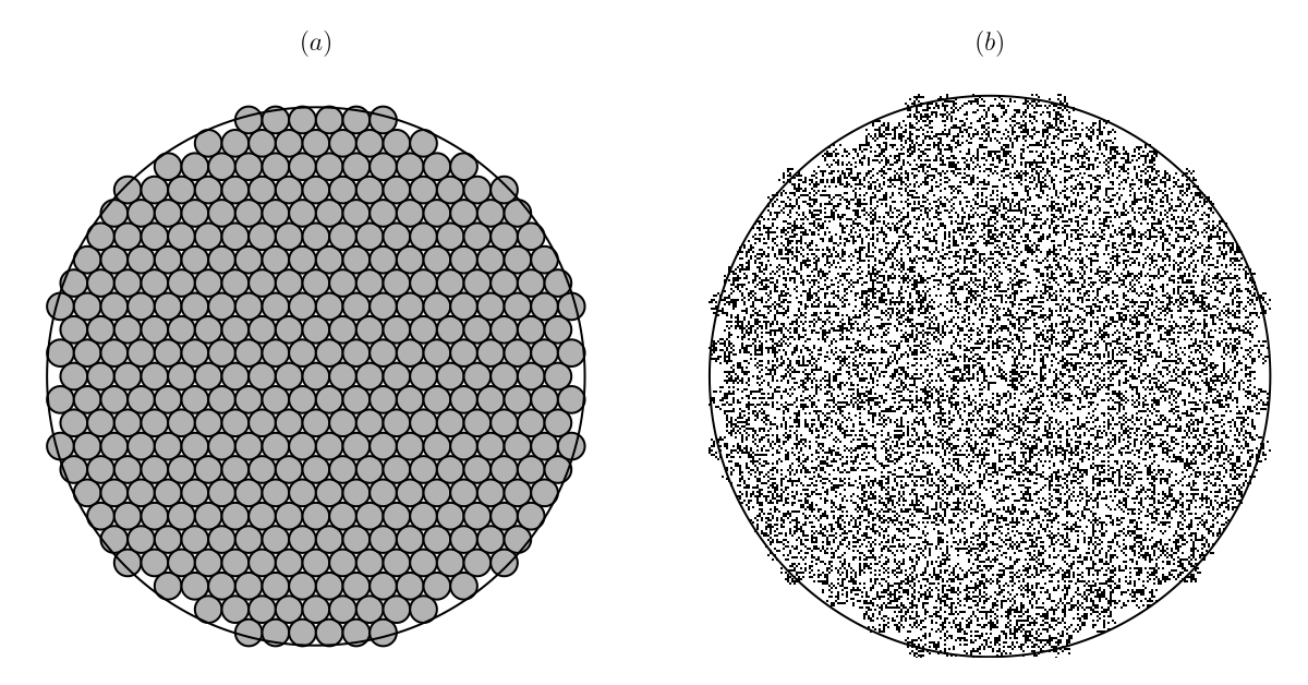
Note that each small disk in Figure 6.1.7 (a) determines a similarity transformation which maps the whole unit disk onto the small disk. If we assume that the similarity neither rotates nor reflects the image, then the similarity is uniquely determined. Thus Figure 6.1.7 (a) describes an iterated function system. The invariant set of this IFS is rendered with a stochastic algorithm in Figure 6.1.7 (b). As we can see, it is close to the whole disk.

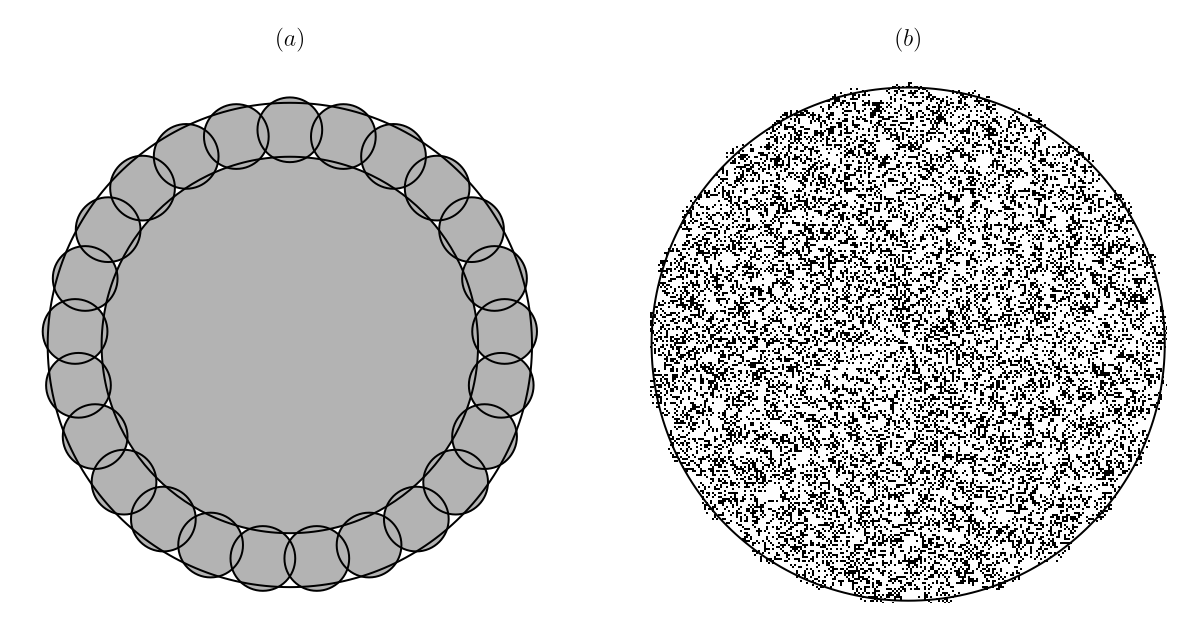
A major problem with the above technique is that it typically yields a large number of transformations. The IFS determined by Figure 6.1.7, for example, has 365 functions. A practical approach which avoids this problem is to try to approximate the image you want with as small a number of affine copies of itself as possible. Such an approach is illustrated for a disk in Figure 6.1.8.

Subsection 6.1.4 Dimension of self-affine sets

Computing the fractal dimension of self-affine sets in general is much harder than for self-similar sets, even assuming the open set condition. We’ll begin by looking at several examples. Our first example is the set \(E\) illustrated in Figure 6.1.9. It consists of four parts scaled by the factor \(1/4\) in the horizontal direction and \(1/2\) in the vertical direction.

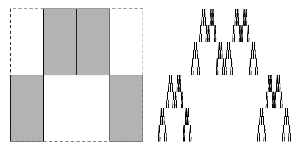
We will compute the box-counting dimension of \(E\text{.}\) To do so, we first cover it with rectangles. By applying the IFS to the unit square \(n\) times, we see that \(4^n\) rectangles of width \(1\left/4^n\right.\) and height \(1\left/2^n\right.\) can cover \(E\text{.}\) This is illustrated for \(n=2\) in Figure 6.1.10.

We need to translate this cover by rectangles into a cover by \(\varepsilon\) mesh squares. A rectangle of width \(1\left/4^n\right.\) and height \(1\left/2^n\right.\) can be decomposed into a stack of \(2^n\) squares of side length \(1\left/4^n\right.\text{,}\) for then the total height of the stack is \(2^n/4^n=1\left/2^n\right.\text{.}\) We now take \(N_{\varepsilon }(E)\) to denote the number of open \(\varepsilon\) mesh squares that intersect \(E\text{.}\) Since the \(n^{\text{th}}\) level approximation generated by the IFS yields \(4^n\) rectangles that can each be decomposed into \(2^n\) squares of side length \(1\left/4^n\right.\text{,}\) we compute \(N_{4^{-n}}(E)=2^n4^n=8^n\text{.}\)

There are a couple of technical points that have been glossed over in this exposition. First, we explicitly stated that \(N_{\varepsilon }(E)\) denotes the number of open \(\varepsilon\) mesh squares that intersect \(E\text{.}\) This allows us to ignore those squares that intersect the set \(E\) at their boundary. As mentioned in chapter 3, this definition is within a constant multiple of the result obtained by using closed \(\varepsilon\) mesh squares and, therefore, yields the correct dimension computation. The other point is more subtle. Clearly, each rectangle generated by the IFS intersects the invariant set \(E\) but how do we know that each of the \(2^n\) sub-squares into which these rectangles were decomposed intersect the set \(E\text{?}\) For this particular example, we can prove that the projection of \(E\) onto the \(y\)-axis is the unit interval, since this is clearly true for each approximation to the set. Using the self-affine structure of the set it can be shown that each of those \(2^n\) sub-squares indeed intersects the set.

To outline an approach for a slightly harder example, consider the self-affine set illustrated back in Figure 6.1.1. We now denote this set by \(E\text{,}\) which consists of \(3^n\) pieces scaled by the factor \(3^{-n}\) in the horizontal direction and \(2^{-n}\) in the vertical direction. Now, there is no single natural choice of a sequence \(\varepsilon _n\) to use in the computation of \(N_{\varepsilon }\text{.}\) Nonetheless, we can estimate \(C_{\sqrt{2}3^{-n}}(E)\text{,}\) the number of sets of diameter \(\sqrt{2}3^{-n}\) required to cover \(E\text{,}\) by using squares of side length \(3^{-n}\text{.}\) Now, the IFS generates \(3^n\) rectangles of width \(3^{-n}\) and height \(2^{-n}\) that cover \(E\text{.}\) In turn, these can be covered with at most \(\left\lceil 3^n/2^n\right\rceil +1\) squares of side length \(3^n\text{.}\) Thus, \(C_{\sqrt{2}3^{-n}}(E)\leq 3^n\left(\left\lceil 3^n/2^n\right\rceil +1\right)\) so

To generate (the same) lower bound for the dimension, we consider packings by balls of radius \(\left.3^{-n}\right/2\) with centers in \(E\text{.}\) Each rectangle generated by the IFS as shown in Figure 6.1.1 stretches vertically along a \(y\) interval of the form \(\left[\frac{i}{2^n},\frac{i+1}{2^n}\right]\text{.}\) As in the previous example, the projection of the portion of \(E\) contained in this rectangle onto the \(y\)-axis is precisely this interval. Thus, we can find points in the intersection of \(E\) and this rectangle with \(y\)-coordinates of the form \(\frac{i}{2^n}+\frac{j}{3^n}\) for \(j=1,2,\ldots ,\left\lfloor 3^n/2^n\right\rfloor\text{.}\) Thus, we can pack at least \(\left\lfloor 3^n/2^n\right\rfloor\) open balls of radius \(\left.3^n\right/2\) into this portion of \(E\text{.}\) A glance at Figure 6.1.1 indicates that we need not worry about lateral intersections between balls coming from different rectangles. Thus, \(P_{\left.3^{-n}\right/2}(E)\geq \left\lfloor 3^n/2^n\right\rfloor\) so

Taking these two results together, we see that \(\dim (E)=\log (9/2)/\log (3)\approx 1.369\text{.}\)

Clearly, it would be nice to have theorem analogous to theorem Theorem 5.4.2 that would allow us to compute the dimension of a self-affine set using a simple formula. Ideally, the formula should hold under reasonably simple hypotheses. While we’ll meet such a formula in the next section, it is not nearly as broadly applicable as theorem Theorem 5.4.2. In our next example, we’ll see that, even if we assume the strong open set condition, that no simple formula can hold.

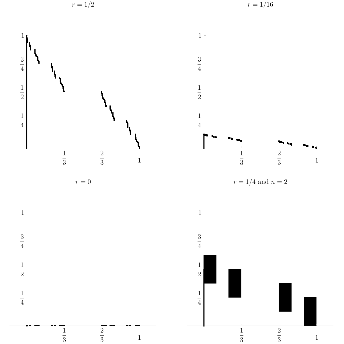
Let \(M\) be the matrix

and consider the IFS with two affine functions

where \(r\) is a real parameter. The invariant set of this IFS for several choices of \(r\) is illustrated in Figure 6.1.11. The dark vertical line segment is the projection of the set onto the \(y\)-axis. There are two key observations to make here. First, for any \(r>0\text{,}\) this projection is a line segment; thus, the dimension of the set must be at least one. Second, for \(r=0\text{,}\) the invariant set is the Cantor set with dimension \(\log (2)/\log (3)\text{,}\) which is strictly less than one. Thus the dimension does not vary continuously with the parameter \(r\) so we can’t expect the dimension to be given by a simple, continuous function of \(r\text{.}\)

Subsection 6.1.5 McMullen carpets

Given the difficulties inherent in computing the dimension of a self-affine set, it's interesting to explore some general situation that forms a simple self-affine set that's not self-similar. One such possibility is the McMullen carpet.

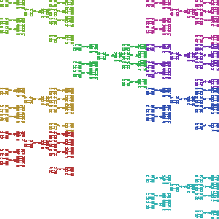
To form a McMullen carpet, choose integers \(m\) and \(n\) such that \(1 \lt m \lt n \text{.}\) Then, decompose the unit square into an \(m\times n\) grid and select a subset of the resulting rectangles. If \(m=3\) and \(n=5\text{,}\) then one such decomposition might look like Figure 6.1.12.

Note that this decomposition implies an iterated function system consisting of \(8\) affine functions - one that maps the unit square onto each of the rectangles that we see in the figure. The attractor of the IFS, in this particular case looks like Figure 6.1.13

There's a formula for the box-counting dimension of a McMullen carpet. In addition to \(m\) and \(n\) as defined above, let \(N\) denote the number of rectangles chosen to form the decomposition and let \(M\) denote the number of columns with at least one chosen rectangle. We'll also denote the attractor by \(C\text{.}\) Then, the box-counting dimension of \(C\) is

Applying this to the example above, we have