Section 1.1 Surprise in Newton's method
Newton's method is a technique to estimate roots of a differentiable function. Invented by Newton in 1669, it remains a stalwart tool in numerical analysis. When used as intended it's remarkably efficient and stable. After a little experimentation, Newton's method yields some surprises that are very nice illustrations of chaos.
Subsection 1.1.1 The basics of Newton's method
Let's begin with a look at the example that Newton himself used to illustrate his method. Let \(f(x)=x^3 - 2x - 5\text{.}\) The graph of \(f\) shown in Figure 1.1.1 seems to indicate that \(f\) has a root just to the right of \(x=2\text{.}\)

Newton figured that, if the root of \(f\) is a little bigger than \(2\text{,}\) then he could write it as \(2+\Delta x\text{.}\) He then plugged this into \(f\) to get
In that last step, since \(\Delta x\) is small, he figures that higher powers of \(\Delta x\) are negligibly small. Thus, he figures that \(-1+10\Delta x \approx 0\) so that \(\Delta x \approx 1/10\text{.}\)
The point is that, if \(2\) is a good guess at a root of \(f\text{,}\) then \(2+1/10 = 2.1\) should be an even better guess. A glance at the graph seems to verify this. Of course, we could then repeat the process using \(2.1\) as the initial guess. We should get an even better estimate. The process can be repeated as many times as desired. This is the basis of iteration.
Subsection 1.1.2 Newton's method in the real domain
Let's take a more general look at Newton's method. The problem is to estimate a root of a real, differentiable function \(f\text{,}\) i.e. a value of \(x\) such that \(f(x)=0\text{.}\) Suppose also that we have an initial guess \(x_0\) for the actual value of the root, which we denote \(r\text{.}\) Often, the value of \(x_0\) will be based on a graph. Since \(f\) is differentiable, we can estimate \(r\) with the root of the tangent line approximation to \(f\) at \(x_0\text{;}\) let's call this point \(x_1\text{.}\) When \(x_0\) is close to \(r\text{,}\) we often find that \(x_1\) is even closer. This process is illustrated in Figure 1.1.2 where it indeed appears that \(x_1\) is much closer to \(r\) than \(x_0\text{.}\)

We now find a formula for \(x_1\) in terms of the given information. Recall that \(x_1\) is the root of the tangent line approximation to \(f\) at \(x_0\text{;}\) let's call this tangent line approximation \(\ell\text{.}\) Thus,
and \(\ell(x_1)=0\text{.}\) Thus, we must simply solve
for \(x\) to get \(x_1 = x_0-f(x_0)/f'(x_0)\text{.}\)
Now, of course, \(x_1\) is again a point that is close \(r\text{.}\) Thus, we can repeat the process with \(x_1\) as the guess. The new, better estimate will then be
The process can then repeat. Thus, we can define a sequence \((x_n)\) recursively by
This process is called iteration and the sequence it generates often converges to the root \(r\text{.}\)
Subsubsection 1.1.2.1 Examples
We now present several examples to illustrate the variety of things that can happen when we apply Newton's method. Throughout, we have a function \(f\) and we defined the corresponding Newton's method iteration function
We then iterate the function \(N\) from some starting point or, perhaps, from several starting points.
Example 1.1.3.
We start with \(f(x)=x^2-2\text{.}\) Of course, \(f\) has two roots, namely \(\pm\sqrt{2}\text{.}\) Thus, we might think, of the application of Newton's method to \(f\) as a tool to find good approximations to \(\sqrt{2}\text{.}\)
First, we compute \(N\text{:}\)
Now, suppose that \(x_0=1\text{.}\) Then,
Note that
so that third iterate is quite close to \(\sqrt{2}\text{.}\)
Note that we've obtained a rational approximation to \(\sqrt{2}\text{.}\) At the same time, it's clear that it would be nice to perform these computations on a computer. In that context, we might generate a decimal approximation to \(\sqrt{2}\text{.}\) Here's how this process might go in Sage:
Note how quickly the process has converged to 12 digits of precision.Of course, \(f\) has two roots. How can we choose \(x_0\) so that the process converges to \(-\sqrt{2}\text{?}\) You'll explore this question computationally in Exercise 1.3.1. It's worth noting, though, that a little geometric understanding can go a long way. Figure 1.1.4, for example, shows us that if we start with a number \(x_0\) between zero and \(\sqrt{2}\text{,}\) then \(x_1\) will be larger than \(\sqrt{2}\text{.}\) The same picture shows us that any number larger than \(\sqrt{2}\) leads to a sequence that converges to \(\sqrt{2}\text{.}\)

Example 1.1.5.
We now take a look at \(f(x)=x^2+3\text{.}\) A simple look at the graph of \(f\) shows that it doesn't even hit the \(x\)-axis; thus, \(f\) has no roots. It's not at all clear what to expect from Newton's method.
A simple computation shows that the Newton's method iteration function is
Note that \(N(1)=-1\) and \(N(-1)=1\text{.}\) In the general context of iteration that we'll consider later, we'll say that the points \(1\) and \(-1\) lie on an orbit of period 2 under iteration of the function \(N\text{.}\)
Sequences of other points seem more complicated so we turn to the computer. Suppose that we change the initial seed \(x_0=1\) just a little tiny bit and iterate with Sage.
Well, there appears to be no particular pattern in the numbers. In fact, if we generate 1000 iterates an plot those that lie within 10 units of the origin on a number line, we get Figure 1.1.6. This is our first illustration of chaotic behavior. Not just because we see points spread all throughout the interval but also because we appeared to have a stable orbit when \(x_0=1\text{.}\) Why should the behavior be so different when we change that initial seed to \(x_0=0.99\text{?}\) 
Example 1.1.7.
Newton's original example had one real root, Example 1.1.3 had two real roots and Example 1.1.5 had no real roots. Let's take a look at an example with lots real roots, namely \(f(x)=\cos(x)\text{.}\)
Generally, the closer your initial seed is to a root, the more likely the sequence starting from that seed is to converge to that root. What happens, though, if we start some place that's not so close to a root? What if we start close to the maximum - near zero? Let's investigate in code.
OK, let's pick this code apart. The inner for loop looks like so:
xi = random()/10
for i in range(8):
    xi = N(xi)
Thus, xi is set to be a random number between \(0\) and \(0.1\text{;}\) the for loop then iterates the Newton's method function in for the cosine from that initial seed 8 times. The outer for loop simply performs this experiment 10 times. After each run of the experiment, we print the resulting \(xi\) - along with the value of the cosine at that point, to check that we're indeed close to a root of the cosine. It's striking that we get 9 different results over 10 runs even though the starting points are so close to one another.
Figure 1.1.8 gives some clue as to what's going on. Recall that we can envision a Newton step for a function \(f\) from a point \(x_i\) by drawing the line that is tangent to the graph of \(f\) at the point \((x_i,f(x_i))\text{.}\) The value of \(x_i\) is then the point of intersection of this line with the \(x\)-axis. Because the slope at the maximum is zero, the value of this point of intersection is very sensitive to small changes. In fact, there are infinitely many roots of the cosine any one of which could be hit by some initial seed in this tiny interval.

Subsection 1.1.3 Newton's method in the complex domain
Let's move now to the complex domain, where even crazier things can happen. To understand this stuff, of course, you'll need a basic understanding of complex numbers but it's really not a daunting amount of information. You'll need to know that a complex number \(z\) has the form
where \(x\) and \(y\) are real numbers (the real and imaginary parts of \(z\)) and \(i\) is the imaginary unit (thus \(i^2=-1\)). You'll also need to know (or accept) that you can do arithmetic with complex numbers and plot them in a plane, called the complex plane. We'll discuss complex variables in a more detail when we jump into complex dynamics more completely.
Subsubsection 1.1.3.1 Cayley's question
In the 1870s, the prolific British mathematician Arthur Cayley (whose name is all over abstract algebra) posed the following interesting question: Given a Suppose that \(p\) is a complex polynomial and \(z_0\) is an initial seed that we might use for Newton's method. Generally, \(p\) will have several roots scattered throughout the complex plane. Is it possible to tell to which of those roots (if any) Newton's method will converge to when we start at \(z_0\text{?}\)
Generally, the closer an initial seed is to a root, the more likely that seed will lead to a sequence that converges to the root. It might be reasonable to guess that the process always converges to the root that is closest to the initial seed. Cayley proved that this is true for quadratic functions but was commented that the general question is much more difficult for cubics. With the power of the computer, there is a very colorful way to explore the question
Algorithm 1.1.9. Coloring basins of attraction for Newton's method.
Given: A function \(f:\mathbb C \to \mathbb C\text{.}\)
-
Choose a rectangle \(R\) in the complex plane with sides parallel to the real and imaginary axes.
The points in \(R\) represent potential initial seeds when applying Newton's method to \(f\text{.}\)
Discretize the rectangle into points of the form
\begin{equation*} z_{0,jk} = (a+j\Delta x) + (b + k\Delta y)k. \end{equation*}-
For each point \(z_{0,jk}\) perform Newton's iteration to generate a sequence \((z_{n,jk})_n\) until one of two things happen:
\(|f(z_{n,jk})| < \varepsilon\text{,}\) where \(\varepsilon\) is some pre-specified small number. We assume that the process has converged to a root; color the initial seed \(z_{0,jk}\) according to which root the process converged to and shade the initial seed according to how many iterates this process took.
The iteration count exceeds some pre-specified bailout; we color the initial seed \(z_{0,jk}\) black.
Let's take a look at a simple, quadratic example.
Example 1.1.10.
Let \(p(z)=z^2+3\text{.}\) We already played with this function in the real case back in Example 1.1.5 and the computer indicated that there might be chaos on the real line. When we allow complex inputs, though, there are two roots - one at \(\sqrt{3}i\) (above the real axis) and one at \(-\sqrt{3}i\) (below the real axis). If the process always converges to the root that is closest to the initial seed, then seeds in the upper half plane should converge to \(\sqrt{3}i\) while seeds in the lower half plane should converge to \(-\sqrt{3}i\text{.}\) We don't have the tools to prove this yet, but we can investigate with Algorithm 1.1.9. The result is shown in Figure 1.1.11.

Now, let's take a look at a classic, cubic example.
Example 1.1.12.
Let \(p(z)=z^3 - 1\text{.}\) As a complex, cubic polynomial, we expect \(p\) to have three roots. It's easy to see that \(z=1\) is a root. This means that \(z-1\) is a factor, which makes it easier to find that
We can then apply the quadratic formula to find that the other two roots are
Note that all three roots can be clearly seen in Figure 1.1.13, which shows the result of Algorithm 1.1.9.
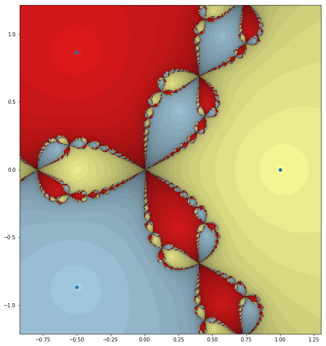
Figure 1.1.13 is just an incredible picture. We can clearly see the three roots of \(p\) and, indeed, if we start close enough to a root we do converge to that root. The boundary between the basins seems to be incredibly complicated, though.
As a final example, let's take a look at the complex cosine.
Example 1.1.14.
Let \(f(z)=\cos(z)\text{.}\) Of course, we played with the real cosine back in Example 1.1.7. There, we saw that in any tiny interval containing zero, an initial seed might converge to any of infinitely many roots. In the complex case, the basins of attraction are shown in Figure 1.1.15, and a zoom is shown in Figure 1.1.16.
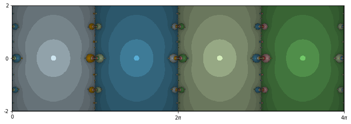
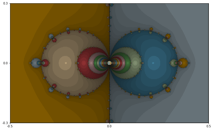
Two more incredible pictures! Note the periodicity in Figure 1.1.15. Each root seems to have its own column of attraction. The boundaries between the basins are again very complicated. In the zoom of Figure 1.1.16, t looks like there's an infinite sequence of circles collapsing on either side of the origin. This agrees with our observations in the real case of Example 1.1.7.
Generating pictures for the Newton's method is great fun. There is an online tool that allows you to generate the basins of attraction for an (almost) arbitrary polynomial here:
https://marksmath.org/visualization/complex_newton/.