Section 5.3 Box-counting dimension
As mentioned earlier, there are many definitions of fractal dimension, all with their own strengths and weaknesses. A major strength of the similarity dimension is that it is very easily computed. A major weakness of the similarity dimension is that it is very restrictive; there are many sets (even very simple sets) which are simply not self-similar. Another weakness is that many people find it to be non-intuitive when compared to the simple definition of equation (5.1.1).
The box-counting dimension has properties that are somewhat complementary to those of the similarity dimension. In particular, it is much more broadly applicable, although harder to compute. In addition, we can show that it yields the right value for most simple sets and it is a more intuitively direct generalization of equation (5.1.1).
Subsection 5.3.1 Definition of box-counting dimension
Throughout this section, \(E\) will denote a non-empty, closed, bounded subset of \(\mathbb{R}^n.\) We wish to associate a notion of dimension with sets at that generality. To do so, we need to think about ways to decompose \(E\) into smaller sets, that aren't necessarily similar to the whole.
Definition 5.3.1. Box covering.
For \(\varepsilon >0,\) the \(\varepsilon\)-mesh for \(\mathbb{R}^n\) is the grid of closed cubes of side length \(\varepsilon\) with one corner at the origin and sides parallel to the coordinate axes. For \(n=2,\) this can be visualized as fine graph paper and we might call an \(\varepsilon\)-mesh cube a square, in that situation. Define \(N_{\varepsilon }(E)\) to be the smallest number of \(\varepsilon\)-mesh cubes whose union contains \(E.\)
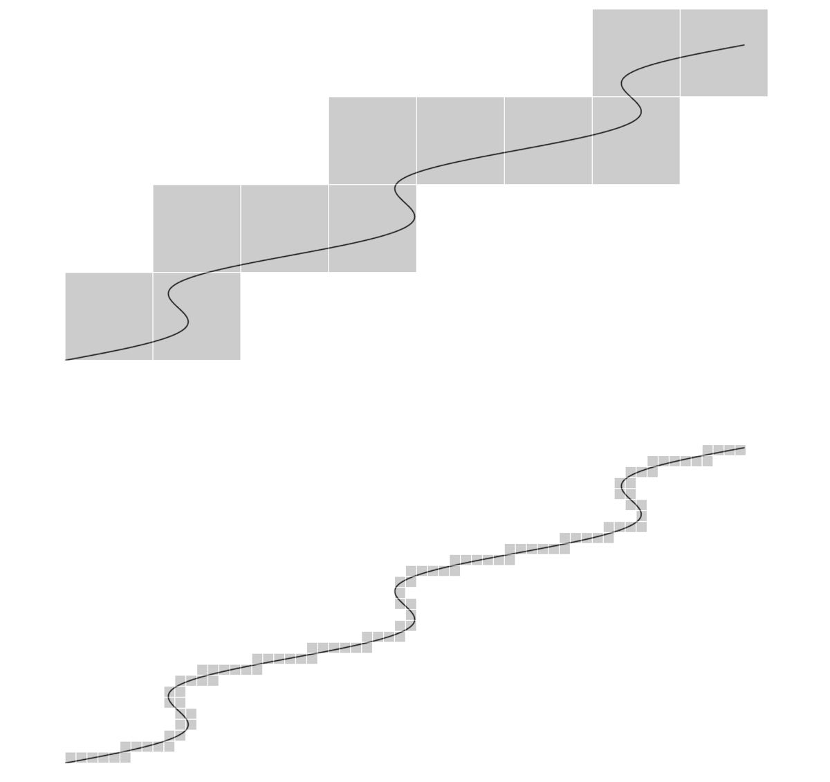
A covering of a smooth curve in the plane by \(\varepsilon\)-mesh squares for two values of \(\varepsilon\) is shown in Figure 5.3.2.
Now, we might think of \(N_{\varepsilon }(E)\) as analogous to \(N_r\) in equation (5.1.1). That leads us to the expression
Definition 5.3.3. Box-counting dimension.
The box-counting dimension \(\dim (E)\) of a non-empty, bounded subset \(E\) of \(\mathbb{R}^n\) is defined by
provided this limit exists.
In fact, we can argue that this should give us the correct dimension of \(1\) whenever \(E\) is a smooth curve with length \(L\) as follows: A glance at Figure 5.3.2 indicates that, for small \(\varepsilon\text{,}\) we expect that
Taking the logarithm of both sides, we find that
so that
as \(\varepsilon\searrow0\text{.}\)
More generally, if
where \(M\) is some measure of size dependent on dimension \(d\) (for example, \(M\) would be area when \(d=2\)), then
as \(\varepsilon\searrow0\text{.}\)
Subsection 5.3.2 Practical computation
While the box-couting dimension is certainly of theoretical importance, it is also of great interest in the natural sciences because it can be estimated fairly easily in a wide variety of situations. We discuss the practical aspects of that computation here.
Before beginning, we should consider that our input is likely to be some sort of raster image approximating some real world object. To be concrete, let's address Mandelbrot's famous question How long is the coast of Britain? This coast, along with a box covering of 241 squares is shown in Figure 5.3.4.
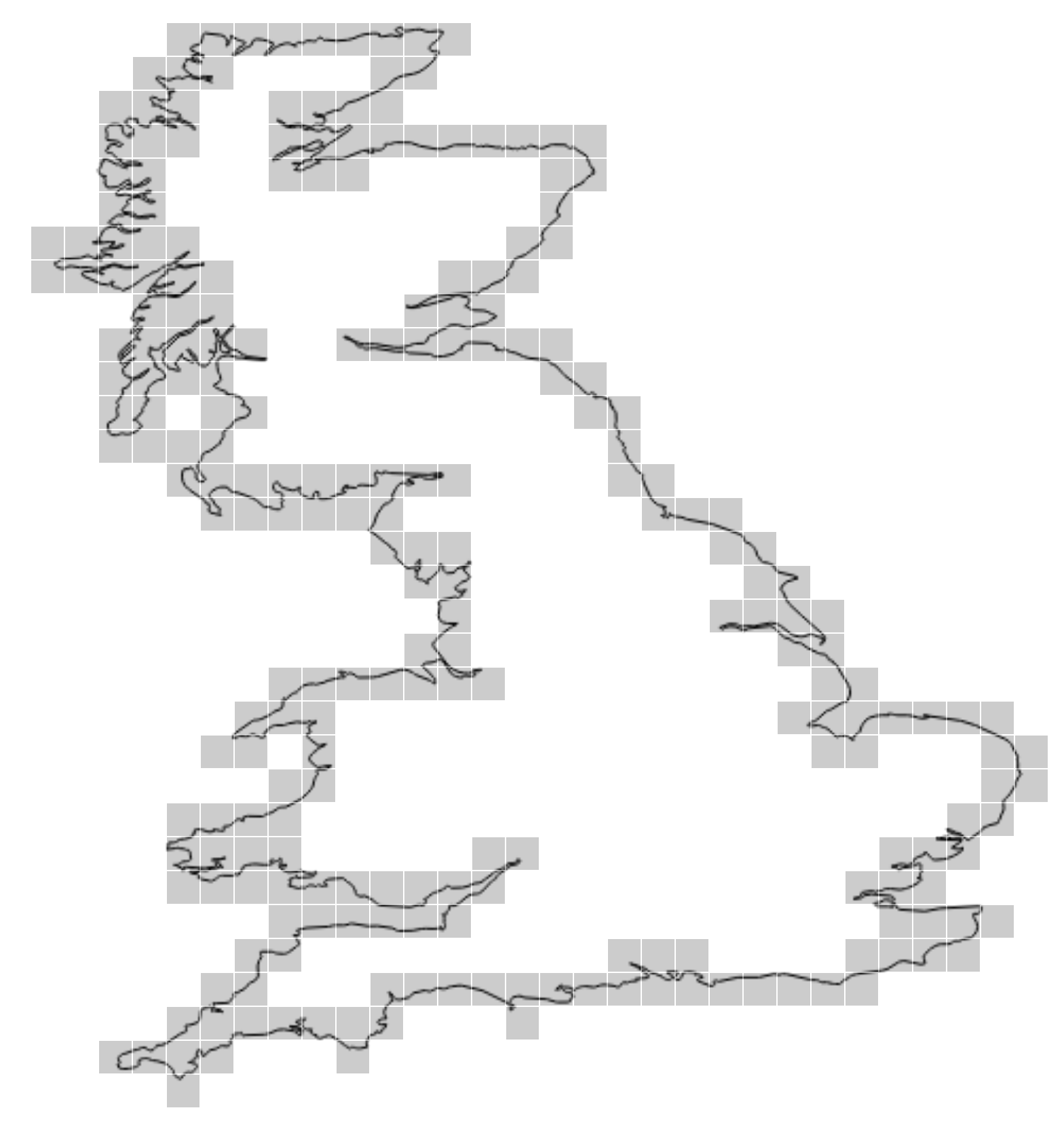
Given this type of input, working straight from the definition to compute \(\log(241)/\log(\text{size})\) is not likely to be fruitful. For one thing, what's size? It doesn't seem like it should matter since dimension should certainly be independent of scale but it certainly would impact our specific estimate. Another issue is that we certainly can't compute a limit as \(\varepsilon\searrow0\) directly, as we have only a finite model. The data for Figure 5.3.4 consists of 3707 lat/lon pairs obtained from Natural Earth.
Another imporant issue is regularity. While self-similar sets can be very convoluted, they also tend to display a great deal regularity. From the standpoint of box-counting dimension, we might expect the relationsip
to hold over a broad range of values.
Here's an approach that accounts for all of these issues. We rewrite the dimension relation in the last equation as
If we suppose that this relationship is good over a wide range of values, then we see that this is the equation of a line indicating the functional dependence of \(\log N_{\varepsilon}(E)\) on \(\log\varepsilon\text{.}\) Furthermore, the dimension arises as the negative slope of that line. Thus, we might use the computer to generate some box-count data of \(N_{\varepsilon}\) as a function of \(\varepsilon\text{,}\) create a loglog plot of that data, and then compute a regression line for the plot. The negative slope should tell us the dimension.
One more question that arises is - how do we best determine values of \(\varepsilon\) for our samples? We'd like to be efficient, yet still be sure that we capture enough data to accurately compute the dimension. While we don't quite have the tools yet, we'll show a bit later in Lemma 5.3.14 that we can choose a sequence of \(\varepsilon\)s that converge down to zero exponentially. An easy choice is therefore \(\varepsilon_n = 2^{-n}\text{.}\)
Example 5.3.5. Dimension of the British coastline.
You can find an implementation of the box-counting algorithm as described here in this Observable notebook; the British coasline example is included there, among several others. The data for that example is shown in Table 5.3.6. Using that data, we can generate Figure 5.3.7 and compute the regression line to be
| \(r\) | 1 | 2 | 4 | 8 | 16 | 32 | 64 | 128 | 256 | 512 |
| \(N_r\) | 3294 | 2099 | 1119 | 542 | 241 | 103 | 39 | 14 | 4 | 1 |

Subsection 5.3.3 Alternative characterizations of box-counting dimension
There are alternative ways to break a more or less arbitrary set into smaller parts that lead to alternative characterization of the resulting dimension. After the limit, the numerical values are the same but the alternative characterizations lead to proofs of nice theoretical properties.
Definition 5.3.8. Diameter.
The diameter of a non-empty, closed, bounded set \(E\subset\mathbb R^n\) is simply the maximum possible distance between any two elements of \(E\text{,}\) i.e.
Definition 5.3.9. \(\varepsilon\)-cover.
Given a non-empty, closed, bounded set \(E\subset\mathbb R^2\) and an \(\varepsilon>0\text{,}\) an \(\varepsilon\)-cover of \(E\) is a collection of closed, bounded sets of diameter at most \(\varepsilon\) whose union contains \(E\text{.}\) We let \(C_{\varepsilon}(E)\) denote the smallest possible number of elements in an \(\varepsilon\)-cover of \(E\text{.}\)
Definition 5.3.10. \(\varepsilon\)-packing.
Given \(\varepsilon >0\text{,}\) an \(\varepsilon\)-packing of \(E\) is a collection of closed, disjoint balls of radius \(\varepsilon\) with centers in \(E\text{.}\) We let \(P_{\varepsilon }(E)\) denote the maximum possible number of balls in an \(\varepsilon\)-packing of \(E.\)
These geometric ideas are illustrated in Figure 5.3.11. In Figure 5.3.11(a), we see a finite collection of points. Figure 5.3.11(b) illustrates a covering of those points, Figure 5.3.11(c) illustrates a packing of the points, and Figure 5.3.11(d) illustrates a box-covering of the points.

We could use any of Definition 5.3.1, Definition 5.3.9, or Definition 5.3.10 to define a notion of dimension. Thus, for the time being, let us write
We'll call these the box-dimension, covering-dimension, and the packing-dimension repsectively.
As it turns out, these definitions are all equivalent. The significance of this fact is that it gives us a lot of flexibility in how we compute dimension. For many sets, \(N_{\varepsilon }(E)\) is the easiest definition to work with. In theoretical situations, \(C_{\varepsilon }(E)\) or \(P_{\varepsilon }(E)\) might be more natural.
Lemma 5.3.12.
IF \(E\) is a non-empty, bounded subset of \(\mathbb{R}^n\text{,}\) then \(\dim _b(E) = \dim _c(E) = \dim _p(E).\)
Proof.
Assume first that the packing dimension is well defined. In other words
exists. We will show that the covering dimension is also well defined and that \(\dim _c(E) = \dim _p(E).\) Suppose we have an \(\varepsilon\)-packing of \(E\) that is maximal in the sense that no more closed \(\varepsilon\)-balls centered in \(E\) can be added without intersecting one of the balls in the packing. Then any point of \(E\) is within a distance at most \(2\varepsilon\) from some center in the packing; otherwise we could add another \(\varepsilon\)-ball to the packing. Thus this \(\varepsilon\)-packing induces a \(4\varepsilon\)-cover of \(E\) obtained by doubling the radius of any ball in the packing as illustrated in figure Figure 5.3.13. In symbols, \(C_{4\varepsilon }(E) \leq P_{\varepsilon }(E).\) It follows that

The expressions on the left and the right both approach \(\dim _p(E)\) as \(\varepsilon \to 0^+\text{.}\) Thus, by the squeeze theorem, the expression in the middle approaches this same value as \(\varepsilon \to 0^+\text{.}\) Of course, this middle limit defines the covering dimension. Thus, the covering dimension exists and \(\dim _c(E) = \dim _p(E).\)
If we assume that the covering dimension exists, then a similar argument shows that the packing dimension exists using the inequality
One can also show that \(\dim _c(E) = \dim _b(E)\) using the inequality
The details are left as an exercise.
In light of Lemma 5.3.12, we will drop the subscripts and refer to the dimension computed using any one of \(N_{\varepsilon }(E),\) \(C_{\varepsilon }(E),\) or \(P_{\varepsilon }(E)\) as the box-counting dimension.
Before looking at an example, we prove another lemma, which simplifies computation considerably.
Lemma 5.3.14.
Let \(\left(\varepsilon _k\right)_k\) be a sequence which strictly decreases to zero and for every \(k\) satisfies \(\varepsilon _{k+1}\geq c \varepsilon _k\text{,}\) where \(c \in (0,1)\) is fixed, and suppose that
Then \(\dim (E)\) is well defined and \(\dim (E) = d.\)
Proof.
Given any \(\varepsilon >0\text{,}\) there is a unique value of \(k\) such that \(\varepsilon _{k+1}\leq \varepsilon <\varepsilon _k\text{.}\) Assuming this relationship between \(\varepsilon\) and \(k\text{,}\) we have
Taking these two inequalities together we have
Now as \(k\to \infty\text{,}\) the expressions on either side of the inequality both approach \(d\text{.}\) Furthermore, \(\varepsilon \to 0^+\) as \(k\to \infty\text{.}\) Thus, by the squeeze theorem,
and this value is \(\dim (E)\) by definition.
Of particular interest are the geometric sequences \(\varepsilon _k = c^k\) where \(c \in (0,1).\) Note that similar results hold for \(N_{\varepsilon }(E)\) and \(P_{\varepsilon }(E)\text{.}\)
Lemma 5.3.14 makes it easy to compute the box-counting dimension of the Cantor set. If \(E\) is the Cantor set, then \(N_{3^{-k}}(E) = 2^k.\) Thus,
It has turned out that the box-counting dimension of the Cantor set is the same as its similarity dimension. As we will see in the next section, this is not by chance. This example should not leave the impression that box-counting dimension is easy to compute. An attempt to compute the box-counting dimension of the generalized Cantor sets should make this clear.