Section 3.7 The components of the Mandelbrot set
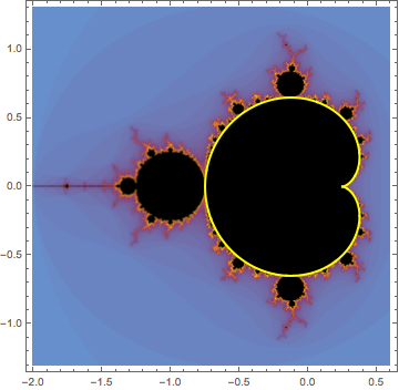
By definition, the Mandelbrot set decomposes the complex parameter plane into two components corresponding to a very coarse decomposition of the types of behavior of \(f_c\text{.}\) A glimpse at figure Figure 3.6.3 (or any of the many images of it available on the web) shows that it consists of rather conspicuous subparts. It appears that there is a large “main cardioid” and that, attached to that main cardioid are a slew of disks or near disks. If we zoom in, we see many smaller copies of the whole set. As it turns out, all these components correspond to particular dynamical behavior. Values of \(c\) chosen from within one component yields functions \(f_c\) with similar qualitative behavior. As \(c\) moves from one component to another, that qualitative behavior changes; we say that a bifurcation occurs. In this section, we'll describe the most conspicuous behavior that we see.
Subsection 3.7.1 Quadratics with super-attractive orbits
We've already seen that \(f_0(z)=z^2\) has a super-attractive fixed point at the origin and that the points \(z_0=0\) and \(z_1=-1\) form a super-attractive orbit of period 2 for \(f_{-1}(z)=z^2-1\text{.}\) We also know, from our work with real iteration, that there is a \(c\) value around \(-1.75\) so that \(f_c\) has a super-attractive orbit of period 3. It turns out that there are two more complex super-attractive period 3 parameters. We can find them with the following Sage code:
Checkpoint 3.7.2.
Locate the points from output of the previous code in the Mandelbrot set and sketch the corresponding Julia sets.
Checkpoint 3.7.3.
Find the complex \(c\)values such that \(f_c\) has a super-attractive orbit of period 4 or 5. Locate these points in the Mandelbrot set and sketch the corresponding Julia sets.
Subsection 3.7.2 The main cardioid
The interior of the main cardioid consists of all those values of \(c\) with the property that \(f_c\) has an attractive fixed point. This can be characterized algebraically as
Now, on the boundary we should have
That is, the fixed point is no longer strictly attractive on the boundary but just neutral. Since any complex number of absolute value 1 can be expressed in the form \(e^{2\pi i t}\text{,}\) this pair of equations can be written without the absolute value:
for some \(t\text{.}\) Taking into account the fact that \(f_c(z) = z^2+c\text{,}\) we get
This system of equations can be solved for \(z\) and \(c\) in terms of \(t\text{.}\) It's not even particularly hard. The second equation yields \(z=e^{2\pi i t}/2\text{.}\) This can be plugged into the first equation to get
This happens to be the parametric representation of a cardioid and is exactly the formula used to generate figure Figure 3.7.4
Subsection 3.7.3 The period two bulb
After the main cardioid, the next largest component is the disk attached to the main cardioid at the point \(c=-3/4\text{.}\) This is, in fact, an actual disk attached at that exact point. We can prove this in much the same way that we derived the formula for the main cardioid, though the algebra is a little more involved.
This disk is known as the period two bulb; every function \(f_c\) where \(c\) is chosen from the period two bulb has an attractive orbit of period two. We can characterize this algebraically by first defining \(F_c(z)=f_c(f_c(z))\text{.}\) A point is then part of an attractive orbit of period 2 for \(f_c\) if
Mimicking the construction of the main cardioid in the period 1 case, we find that \(z\) and \(c\) must satisfy
for some \(t\text{.}\) Taking into account the fact that \(F_c(z) = (z^2+c)^2+c\text{,}\) we get
While clearly this is a bit more involved than the period one case, a computer algebra system makes quick work of it. Listing Listing 3.7.5 shows how to solve this system with Mathematica and listing Listing 3.7.6 shows how to solve this system with Sage.
f[c_][z_] = z^2 + c;
F[c_][z_] = Nest[f[c], z, 2];
eqs = {F[c][z] == z, F[c]'[z] == Exp[2 Pi*I*t]};
Expand[c /. Last[Solve[eqs, {c, z}]]]
(* Out:
	-1 + E^((2*I)*Pi*t)/4
*)
Note that both program listings Listing 3.7.5 and Listing 3.7.6 yield the result
which parametrizes a circle of radius \(1/4\) centered at the point \(-1\text{.}\)
Also, it's certainly feasible to solve this system by hand. The expression \(F_c(z)-z\) factors so that the system really just involves a couple of quadratics. Use of the computer will be quite convenient as we move into higher order examples, though.
Subsection 3.7.4 The Mandelbrot set as a bifurcation locus
We've now got a solid understanding of the period 1 component of the Mandelbrot set (the main cardioid) and the period 2 component (the period 2 bulb). The period 2 component is called a “bulb” because it is directly attached to the main cardioid. Indeed, using our parametrizations, you can show easily enough that the point \(c=-3/4\) lies on both the boundary of the main cardioid and on the boundary of the period 2 component. Note that, for this value of \(c\text{,}\) \(f_c\) has a neutral fixed point at \(z=-1/2\text{.}\) As \(c\) moves from the main cardioid, through the point \(-3/4\text{,}\) and into the period 2 bulb, the function \(f_c\) undergoes a bifurcation - that is a qualitative change in the global dynamics of the function. More specifically, \(f_c\) changes from having an attractive fixed point to having an attractive orbit of period 2. This is very much like the bifurcation diagram that we saw when studying real iteration. In fact:
The geometric relationship between the Mandelbrot set and the bifurcation diagram is made explicit in figure Figure 3.7.7.
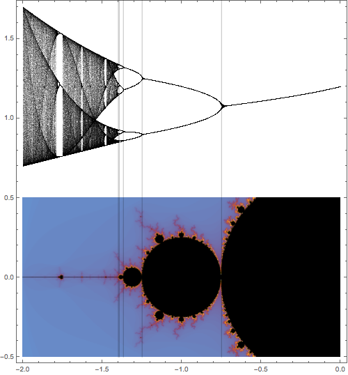
Figure Figure 3.7.7 shows only how the Mandelbrot set aligns with the real bifurcation diagram. There is really much more to the picture, though. All the visible components of the Mandelbrot set correspond to distinct, qualitative behavior. As \(c\) moves within one component, the qualitative behavior of \(f_c\) stays the same. More precisely, any two values of \(c\) chosen from the same component will have attractive orbits of the same period. As \(c\) moves from any component of the Mandelbrot set to another in the complex plane, \(f_c\) undergoes a bifurcation - period doubling, tripling, or whatever. If \(c\) exits the Mandelbrot set, \(f_c\) undergoes a more complicated type of bifurcation.
This all suggests another way to draw the Mandelbrot set. We iterate from the critical point zero, as in algorithm Algorithm 3.6.2, but we stop iteration whenever we find some sort of attractive behavior. We then color the point \(c\) according to the period of the orbit we find and shade it according to how long it took to detect the periodicity. The result is shown in figure Figure 3.7.8.
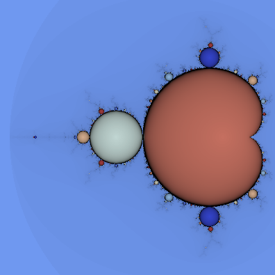
Subsection 3.7.5 Higher period bulbs
Figure Figure 3.7.8 shows that there are lots of disk-like bulbs attached to the main cardioid. As \(c\) moves from the main cardioid into one of these bulbs, \(f_c\) bifurcates from having an attractive fixed point, to an orbit of period \(q\) for some integer \(q \gt 1\text{.}\) After the period 2 bulb, the two next largest bulbs near the top and bottom of the main cardioid are period 3 bulbs. The other bulbs have larger period still.
Let's try to gain a quantitative understand of the nature of these bulbs. To do so, we re-consider our description of the main cardioid from subsection Subsection 3.7.2. Again, the interior of the main cardioid can be characterized algebraically as
More generally, though, we can obtain a fixed point with any given multiplier \(\gamma\) that we like by solving
If we solve this system for \(c\) and \(z\text{,}\) we obtain
Thus, \(f_c\) has a fixed point with multiplier \(\gamma\) at \(\gamma/2\) when \(c=(2\gamma - \gamma^2)/4\text{.}\)
Let us now define \(c(\gamma) = (2\gamma - \gamma^2)/4\) and consider the image of rays of the form \(r\exp(2\pi i \theta)\text{,}\) where \(\theta\) is fixed and \(0\leq r \leq 1\text{.}\) These should all lie within the main cardioid and stretch from zero to a point on the boundary of the cardioid. Some of these are plotted in figure Figure 3.7.9.
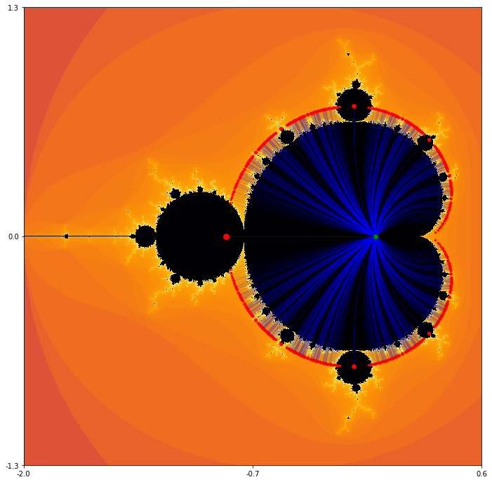
Note that the rays shown in figure Figure 3.7.9 all correspond to rational values of \(\theta\) and, as it appears, a periodic bulb is attached to the main cardioid at every rational ray. Even more is true - if \(\theta=p/q\text{,}\) then the bulb attached to the main cardioid at the point \(c(\exp(2\pi i \theta))\) has period \(q\) and rotation number \(p\text{.}\)
To understand this, recall that \(c(\gamma)\) is built specifically so that \(f_{c(\gamma)}\) will have multiplier \(\gamma\text{.}\) So, what happens to the attractive orbits of \(f_c(\gamma)\) for
for a fixed rational value of \(\theta\) as \(r\) moves from zero up to one and even just a little bit past? For \(r \lt 1\text{,}\) \(f_c\) has an attractive fixed point. For \(r=1\text{,}\) \(f_c\) has a neutral fixed point with multiplier \(\gamma=\exp(2\pi i \theta)\text{.}\) Note that the geometric effect of multiplying by this particular value of \(\gamma\) is to rotate through the angle \(2\pi\theta=2\pi p/q\text{.}\) If we do this \(q\) times, we've rotated through the angle \(2\pi\theta=2\pi p\text{,}\) which returns to where we started. We might expect an attractive orbit of period \(q\text{;}\) we don't have it yet because the origin still in the basin of the neutral fixed point. Once \(r \gt 1\text{,}\) that fixed point becomes slightly repulsive and the attractive orbit of period \(q\) appears.
Note that each of these bulbs has further bulbs sprouting off and similar considerations apply.
Subsection 3.7.6 Baby-brots
There are loads of little copies of the Mandelbrot set strewn throughout. For the time being, I'll refer to this Math.StackExchange post: http://math.stackexchange.com/questions/404066/.