Digraph Iterated Function Systems

Section 6.2 Digraph Iterated Function Systems

Self-affinity generalizes self-similarity by expanding the class of functions in the iterated function system. In this section, we’ll generalize the concept of an iterated function system itself.

Subsection 6.2.1 Motivating example

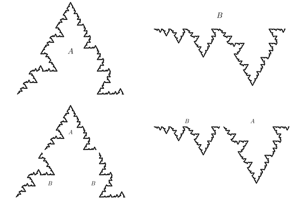
Rather than considering a single set composed of copies of itself, we consider a collection of sets each composed of copies of sets chosen from the collection. As an example, consider the two curves \(A\) and \(B\) shown in Figure 6.2.1. The curve \(A\) is composed of 1 copy of itself, scaled by the factor \(1/2\text{,}\) and 2 copies of \(B\text{,}\) rotated by \(\pm 60^{\circ}\) and scaled by the factor \(1/2.\) The curve \(B\) is composed of 1 copy of itself, scaled by the factor \(1/2,\) and 1 copy of \(A\text{,}\) reflected and scaled by the factor \(1/2.\) The curves \(A\) and \(B\) are called digraph self-similar sets and may be described using a digraph iterated function system or digraph IFS.

Subsection 6.2.2 The definition of a digraph IFS

The first ingredient to define a digraph IFS is a directed multi-graph. A directed multi-graph \(G\) consists of a finite set \(V\) of vertices and a finite set \(E\) of directed edges between vertices. We call \(G\) a multi-graph because we allow more than one edge between any two vertices. Figure Figure 6.2.2 shows the directed multi-graph for the curves \(A\) and \(B\text{.}\) There are two edges from vertex \(A\) to vertex \(B\) and one edge from vertex \(A\) to itself since \(A\) consists of two copies of \(B\) together with one copy of itself. Similarly, there is one edge from vertex \(B\) to vertex \(A\) and one edge from vertex \(B\) to itself since \(B\) consists of one copy of \(A\) together with one copy of itself.

Figure 6.2.2. The digraph for the curves

Note that the edges in figure Figure 6.2.2 are labeled. The subscript of each label indicates the initial and terminal vertices of the corresponding edge. We obtain a digraph IFS from a directed multi-graph by associating a contraction \(f_e\) with each edge \(e\) of the digraph. Often, the functions will be affine functions or, even, similarities. The digraph IFS for the digraph curves \(A\) and \(B\) is generated from figure Figure 6.2.2 by associating a similarity transformation with each edge of the digraph. We can list them as follows, using the notation of Subsection 4.5.1.

\begin{align*} f_{aa} \amp= T_{\langle 1/4, \sqrt{3}/4 \rangle} \circ S_{1/2} \\ f_{ab} \amp= R_{60^{\circ}} \circ S_{1/2}\\ g_{ab} \amp= T_{\langle 3/4, \sqrt{3}/4 \rangle} \circ R_{-60^{\circ}} \circ S_{1/2}\\ f_{ba} \amp= T_{\langle 1/2, 0 \rangle} \circ F_{\langle 0,1 \rangle} \circ S_{1/2}\\ f_{bb} \amp= S_{1/2} \end{align*}

The functions associated with the edges indicate how the large sets map onto the constituent parts. For example, the function \(f_{ab}\) maps the set \(B\) onto the lower left portion of the set \(A\text{.}\) To make this type of statement for the general digraph IFS, we need to develop some notation associated with digraph iterated function systems. Given two vertices, \(u\) and \(v\text{,}\) we denote the set of all edges from \(u\) to \(v\) by \(E_{u v}.\) A path through \(G\) is a finite sequence of edges so that the terminal vertex of any edge is the initial vertex of the subsequent edge. A loop through \(G\) is a path which starts and ends at the same vertex. \(G\) is called strongly connected if for every \(u\) and \(v\) in \(V\text{,}\) there is a path from \(u\) to \(v\text{.}\) We denote the set of all paths of length \(n\) with initial vertex \(u\) by \(E_u^n.\) A digraph IFS is called contractive if the product of the scaling factors in any closed loop is less than 1. Theorem 4.3.5 of [Edgar 1990] states that for any contractive digraph IFS, there is a unique set of non-empty, compact sets \(K_v,\) one for every \(v\) in \(V,\) such that for every \(u\) in \(V,\)

\begin{equation} K_u = \underset{v\in V,e \in E_{uv}}{\bigcup } f_e\left(K_v\right).\label{eq-digraphEquation}\tag{6.2.1} \end{equation}

Such a collection of sets is called the invariant list of the digraph IFS and we will refer to its members as digraph fractals. In general, if \(e\in E_{uv}\text{,}\) then \(f_e\) maps \(K_v\) into \(K_u\text{.}\) Thus the functions of the digraph IFS map against the orientation of the edges. Also note that an IFS is the special case of a digraph IFS with one vertex and theorem 4.3.5 of [Edgar 1990] is a generalization of the statement that a unique invariant set exists for a contractive IFS.

To clarify equation (6.2.1), let’s write it down for the specific case of the digraph curves \(A\) and \(B\text{.}\) There is one equation for each vertex, thus in this case, equation (6.2.1) denotes a pair of equations. Substituting \(u=A\) then \(u=B\) we obtain the two equations

\begin{align*} A \amp= f_{aa}(A) \bigcup f_{ab}(B) \bigcup g_{ab}(B)\\ B \amp= f_{ba}(A) \bigcup f_{bb}(B) \end{align*}

Subsection 6.2.3 Digraph tools

Subsection 6.2.4 Computing dimension

Our objective in this section is to develop an intuitive understanding of the dimension computation for digraph fractals. As with self-similar sets, the digraph IFS generates efficient covers of the digraph fractals and the rate of growth of the number of sets in these covers indicates the dimension of the set.

Consider, for example, our digraph self-similar curves and the simple coverings by triangles as shown in Figure 6.2.3. In the top row, we see a level zero cover by triangles of diameter 1. Now, if we apply the digraph IFS to the pair of triangles, we obtain the finer covering shown at level one. The sets in these covers all have diameter 1/2. Iterating again, we obtain covers by sets of diameter 1/4, as shown at level two.

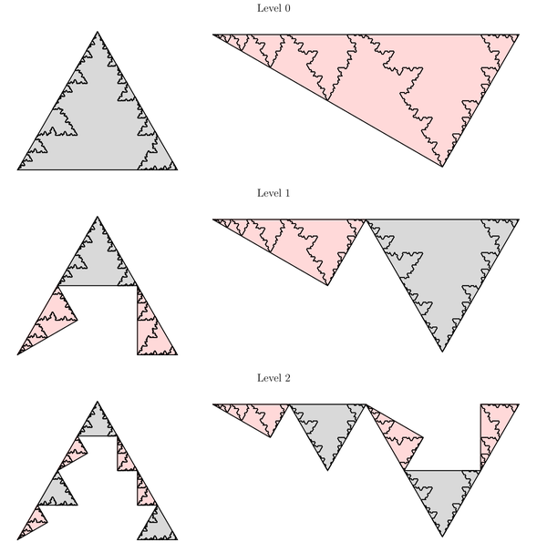
Figure 6.2.3. Covers of the digraph fractal curves

At the \(n^{\text{th}}\) iteration, we obtain covers of \(A\) and \(B\) by sets of diameter \(2^{-n}\text{;}\) we can count the number of sets in these to estimate \(N_{2^{-n}}\left(A\right)\) and \(N_{2^{-n}}\left(B\right)\text{.}\) The key to doing so efficiently is to realize that each set in either cover at the \(n^{\text{th}}\) level corresponds to a path of length \(n\) through the digraph for the sets. Furthermore, the number of such paths may be computed by summing the terms in the \(n^{\text{th}}\) power of the adjacency matrix of the digraph. To see this, let \(A\) denote the adjacency matrix for the digraph. Thus, for our example,

\begin{equation*} A=\left( \begin{array}{cc} 1 & 2 \\ 1 & 1 \\ \end{array} \right). \end{equation*}

Recall that the entry in row \(i\) and column \(j\) denotes the number of edges (or paths of length one) from the \(i^{\text{th}}\) vertex to the \(j^{\text{th}}\text{.}\) Now consider

\begin{equation*} A^2=\left( \begin{array}{cc} 1 & 2 \\ 1 & 1 \\ \end{array} \right)\left( \begin{array}{cc} 1 & 2 \\ 1 & 1 \\ \end{array} \right)=\left( \begin{array}{cc} 1+2 & 2+2 \\ 1+1 & 2+1 \\ \end{array} \right)=\left( \begin{array}{cc} 3 & 4 \\ 2 & 3 \\ \end{array} \right). \end{equation*}

The entry in row \(i\) and column \(j\) of \(A^2\) is the dot product of the \(i^{\text{th}}\) row of \(A\) with the \(j^{\text{th}}\) column and represents the number of paths of length \(2\) from the \(i^{\text{th}}\) vertex to the \(j^{\text{th}}\text{;}\) the \(k^{\text{th}}\) term in that sum represents the number of paths through vertex \(k\text{.}\) It follows from induction that the entry in row \(i\) and column \(j\) of \(A^n\) represents the number of paths of length \(n\) from vertex \(i\) to vertex \(j\text{.}\)

Now consider the vector \(v_n=A^n1\text{,}\) where \(1\) represents the vector of ones. In our example,

\begin{equation*} A^n1=\left( \begin{array}{cc} 1 & 2 \\ 1 & 1 \\ \end{array} \right)^n\left( \begin{array}{c} 1 \\ 1 \\ \end{array} \right). \end{equation*}

The \(i^{\text{th}}\) element of this vector is the sum of the \(i^{\text{th}}\) row of \(A^n\) and represents the number of sets in the \(n^{\text{th}}\) level cover of the \(i^{\text{th}}\) digraph fractal. It turns out that the entries of \(v_n\) grow exponentially at the rate \(\lambda ^n\text{,}\) where \(\lambda\) is the largest eigenvalue of \(A\text{.}\)

These computations suggest that the common dimension of the digraph fractal curves is \(\log (\lambda )/\log (2)\text{,}\) where \(\lambda =1+\sqrt{2}\) is the largest eigenvalue of \(A\text{.}\)