Parameterized families of functions

Section 2.7 Parameterized families of functions

Rather than explore the behavior of a single function at a time, we can introduce a parameter and explore the range of behavior that arises in a whole family of functions.

Subsection 2.7.1 Examples of parameterized families

Two important examples of parameterized families of functions are

The quadratic family: \(f_c(x)=x^2+c\)
The logistic family: \(f_{\lambda}(x)=\lambda x(1-x)\)

The cobweb plots shown back in Figure 2.3.1 are all chosen from the logistic family with \(\lambda=2.8\text{,}\) \(\lambda=3.2\text{,}\) and \(\lambda=4\text{.}\) Even in those three pictures with graphs that look so very similar, we see three different types of behavior: an attractive fixed point, an attractive orbit of period two, and chaos (which can be given a very technical meaning).

Figure 2.7.1 shows some cobweb plots for the quadratic family of functions. Note that the behavior we see is very similar to the behavior we see for the logistic family - a fact that will become more understandable once we study conjugacy in section Section 2.8

Figure 2.7.1. Some cobweb plots for the quadratic family

Subsection 2.7.2 The bifurcation diagram

A fabulous illustration of the types of behavior that can arise in a family of functions indexed by a single real parameter and each with a single critical point can be generated as follows: For each value of the parameter, compute a large number points of the orbit of the critical point (maybe 1000 iterates). Since we're interested in long term behavior, rather than any transient behavior, discard the first few iterates (maybe 100). Then, plot the remaining points in a vertical column at the horizontal position indicated by the parameter.

If we do this systematically for the quadratic family, plotting the columns to generate the bifurcation diagram, we get Figure 2.7.2

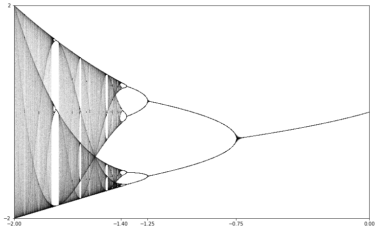
Figure 2.7.2. The bifurcation diagram for the quadratic family

We can interpret this diagram as follows:

For \(-0.75 < c < 0\text{,}\) there is an attractive fixed point.
For \(-1.25 < c < -0.75\text{,}\) there is an attractive orbit of period \(2\text{.}\)
As \(c\) passes from just above \(-0.75\) to just below \(-0.75\text{,}\) the dynamics of \(f_c\) undergo a bifurcation.
For \(c\) just a little less than \(-1.25\text{,}\) there is an attractive orbit of period four. This orbit bifurcates soon into an attractive orbit of period 8. It appears that this behavior continues as \(c\) decreases.
For \(c\) somewhere around \(c\approx -1.4\text{,}\) the period doubling appears to stop and we get more complicated behavior.

Generally, a bifurcation occurs at a parameter value \(c=c_0\) if the global dynamical behavior of the function \(f_c\) undergoes some qualitative change as \(c\) passes through \(c_0\text{.}\) There are number of different types of bifurcations that can occur, depending on the nature of the qualitative behavior under consideration. The bifurcations that are evident in Figure 2.7.2 in the range \(-1.4 < c < 0\) are called period doubling bifurcations.

Subsection 2.7.3 The period doubling cascade

Let's work towards a deeper, theoretical understanding of the period doubling that we see in the bifurcation diagram of Figure 2.7.2. Again, we are dealing with the family of functions \(f_c(x) = x^2+c\text{.}\) For \(c\) just a bit larger than \(-0.75\) it appears that we have an attractive fixed point while, for \(c\) just a bit smaller than \(-0.75\text{,}\) it appears that we have an attracting orbit of period two. Why, exactly does this happen?

First, let's explore the fixed points of \(f_c\text{;}\) we can find them by solving \(f_c(x)=x\text{:}\)

\begin{equation*} x^2+c = x \: \Longleftrightarrow \: x^2-x+c = 0. \end{equation*}

Applying the quadratic formula, we find

\begin{equation*} x = \frac{1\pm\sqrt{1-4c}}{2}. \end{equation*}

For \(c < 1/4\text{,}\) we have two real fixed points but a glance at the graphs from Figure 2.7.1 shows that it's the smaller of these two fixed points we're interested in. Of course, \(f'(x)=2x\text{,}\) so the value of the derivative at the smaller fixed point is \(1-\sqrt{1-4c}\text{.}\) Plugging \(c=-3/4\) into this formula, we find that this is \(-1\text{.}\) For \(c\) slightly larger than \(-3/4\text{,}\) this is bigger than \(-1\) and for \(c\) slightly smaller than \(-3/4\text{,}\) this is smaller than \(-1\text{.}\) This explains why we have an attractive fixed point for \(c\) slightly larger than \(-3/4\) that is no longer attractive once \(c\) passes below \(-3/4\text{.}\)

Now, we ask - why does the attractive orbit of period two appear as the attractive fixed point disappears? To see this, we consider the function

\begin{equation*} F_c(x) = f_c\circ f_c(x) = (x^2+c)^2+c = x^4 + 2cx^2+(c^2+c). \end{equation*}

We are interested in the fixed points, thus we must solve

\begin{equation} x^4 + 2cx^2+(c^2+c) = x \: \text{ or } \: x^4 + 2cx^2 - x + (c^2+c) = 0.\label{equation-f_squared}\tag{2.7.1} \end{equation}

Here is an observation that helps us factor this polynomial: Any point that is fixed by \(f_c\) must also be fixed by \(F_c\text{.}\) Thus, we expect \(x^2+c-x\) to be a factor of the polynomial in (2.7.1). Using this, we find that

\begin{equation*} x^4 + 2cx^2 - x + (c^2+c) = (x^2 - x + c)(x^2 + x + c + 1). \end{equation*}

We can then apply the quadratic formula to get the two new fixed points of \(F_c\text{,}\) namely

\begin{equation*} x = \frac{-1 \pm \sqrt{1-4(c+1)}}{2} = \frac{-1 \pm \sqrt{-(3+4c)}}{2}. \end{equation*}

These two points form an orbit of period two for \(f_c\text{.}\) Since \(f_c'(x)=2x\) we can multiply those points by two and multiply the results to get the multiplier for the orbit. The result is:

\begin{equation*} (-1+\sqrt{-(3+4c)})(-1-\sqrt{-(3+4c)}) = 4+4c. \end{equation*}

When \(c=-3/4\text{,}\) the multiplier is \(1\text{.}\) For \(c\) a little less than \(-3/4\text{,}\) the multiplier is a little less than one. Hence the orbit has become attractive.

A nice way to visualize this is to plot \(f_c^2\) together with \(f_c\) and \(y=x\) on the same set of axes for a few different choices of \(c\text{.}\) This is shown in Figure 2.7.3 where we can see exactly how The fixed point went from attractive to repulsive while an attractive orbit of period two showed up as \(c\) passed below \(-0.75\text{.}\)

Note that our cobweb tool allows you to plot iterates of \(f\) on the plot to assist in this type of analysis.

Checkpoint 2.7.4.

Consider the logistic family \(f_{\lambda}(x) = \lambda x(1-x)\text{.}\)

Using our cobweb tool

Subsection 2.7.4 The critical curves

A close look at Figure 2.7.2 seems to indicate the presence of curves lending structure to the diagram. These are the so-called critical curves.

Definition 2.7.5.

Let \(f_{\alpha}\) be a parameterized family of functions, each with a single critical point \(c_{\alpha}\text{.}\) The \(n^{\text{th}}\) critical curve is defined by \(f_{\alpha}^n(c_{\alpha})\text{,}\) which is a polynomial in \(\alpha\)

For the quadratic family \(f_{c}(x)=x^2+c\text{,}\) the \(n^{\text{th}}\) critical curve is the polynomial \(f_c^n(0)\text{,}\) which is a polynomial in \(c\text{.}\) The first few critical polynomials are

\begin{align*} f_c^0(0) \amp= 0 \\ f_c^1(0) \amp= c \\ f_c^2(0) \amp= c^2+c \\ f_c^3(0) \amp= (c^2 + c)^2 + c \\ f_c^4(0) \amp= ((c^2 + c)^2 + c)^2 + c \end{align*}

If we plot a few of these on top of the bifurcation diagram, we get Figure 2.7.6.

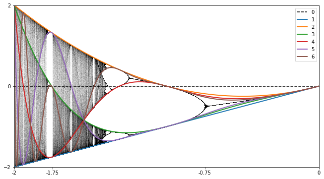
Figure 2.7.7 Gives an indication of how the critical curves form. The dashed parallel lines on either side of the horizontal \(c\)-axis define a region in the plane of the bifurcation diagram. The image of those lines under application of \(f_c^n\) are shown for \(n=1,2,3\) in the figure, together with the corresponding critical curve. As we see, the region bound between the original horizontal lines is mapped by \(f_c^n\) to a much smaller region on one side of the \(n^{\text{th}}\) critical curve. Thus, there is a higher density of points on one side of the each critical curve.

Subsection 2.7.5 Periodic windows

Amongst the chaos apparent within the bifurcation diagram, there appear to be a number periodic windows - a range of parameter values where an attractive periodic orbit dominates the behavior. The largest one appears in Figure 2.7.6 just to the left of \(c=-1.75\) where the third (green) critical curve crosses the horizontal \(c\)-axis. This is the so-called period three window.

Note that the critical curves seem to cross the horizontal \(c\)-axis at exactly the locations of the periodic windows. Corollary 2.5.3 explains why. Note that \(f_c^n(0)\) crosses the horizontal axis exactly when \(f_c^n(0)=0\text{.}\) Thus, \(0\) is periodic for \(f_c\) with a period that divides \(n\text{.}\)

When \(n=3\text{,}\) for example, this leads to the equation

\begin{equation*} (c^2 + c)^2 + c = 0. \end{equation*}

We can find all real roots of this polynomial using the following Sage code:

The value of about \(-1.75\) agrees with our observations. The value of zero occurs because zero is a fixed point of \(f_0\) and, therefore, of \(f_0^3\) as well.

An alternative way to shed light on the sudden occurrence of the period three window is to use cobwebplots as shown in Figure 2.7.8. In that figure on the left, we see the cobweb plot for \(c=-1.6\) together with the \(3^{\text{rd}}\) iterate \(f_{-1.6}^3\) of \(f\text{.}\) The key observation is that the graph of \(f_{-1.6}^3\) completely misses the line \(y=x\text{.}\) Thus, there is no orbit of period three for \(c=-1.6\text{.}\) By the time \(c=-1.76\) on the right figure, there is such an orbit.

Figure 2.7.8. The occurence of the period 3 window

Note that our interactive cobweb tool can be used to explore this further: https://marksmath.org/visualization/cobwebs/