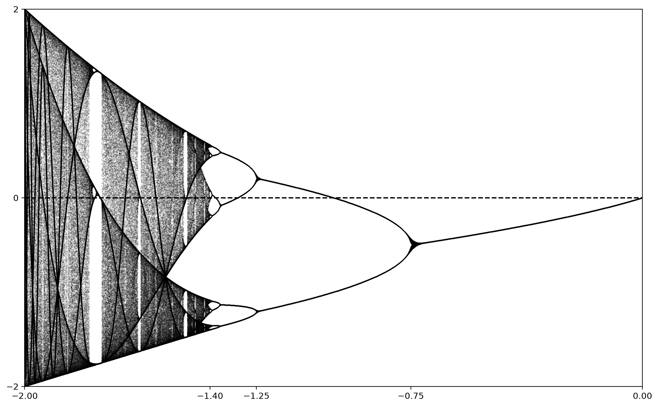
Let \(f_{\alpha}\) be a parameterized family of functions, each with a single critical point \(c_{\alpha}\text{.}\) The \(n^{\text{th}}\) critical curve is defined by \(f_{\alpha}^n(c_{\alpha})\text{,}\) which is a polynomial in \(\alpha\)
For the quadratic family \(f_{c}(x)=x^2+c\text{,}\) the \(n^{\text{th}}\) critical curve is the polynomial \(f_c^n(0)\text{,}\) which is a polynomial in \(c\text{.}\) The first few critical polynomials are
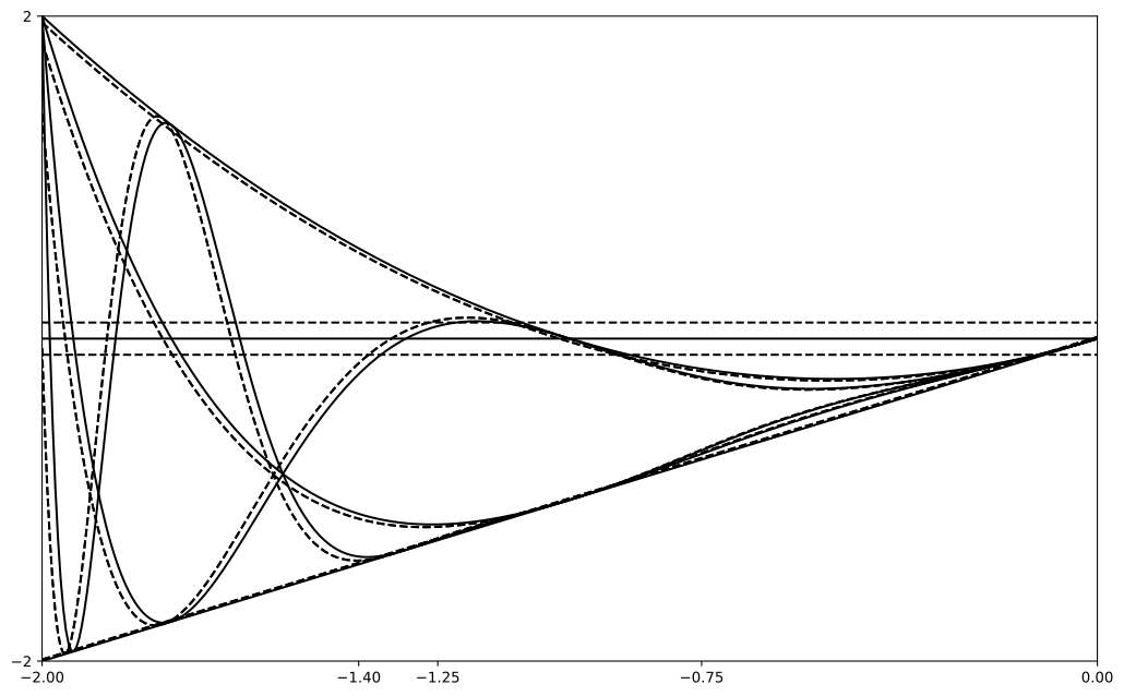
Figure 2.33 Gives an indication of how the critical curves form. The dashed parallel lines on either side of the horizontal \(c\)-axis define a region in the plane of the bifurcation diagram. The image of those lines under application of \(f_c^n\) is shown for \(n=1,2,3\) in the figure, together with the corresponding critical curve. As we see, the region bound between the original horizontal lines is mapped by \(f_c^n\) to a much smaller region on one side of the \(n^{\text{th}}\) critical curve. Thus, there is a higher density of points on one side of each critical curve.