Subsection 2.7.2 The bifurcation diagram
A fabulous illustration of the types of behavior that can arise in a family of functions indexed by a single real parameter and each with a single critical point can be generated as follows: For each value of the parameter, compute a large number of points of the orbit of the critical point (maybe 1000 iterates). Since we’re interested in long term behavior, rather than any transient behavior, discard the first few iterates (maybe 100). Then, plot the remaining points in a vertical column at the horizontal position indicated by the parameter.
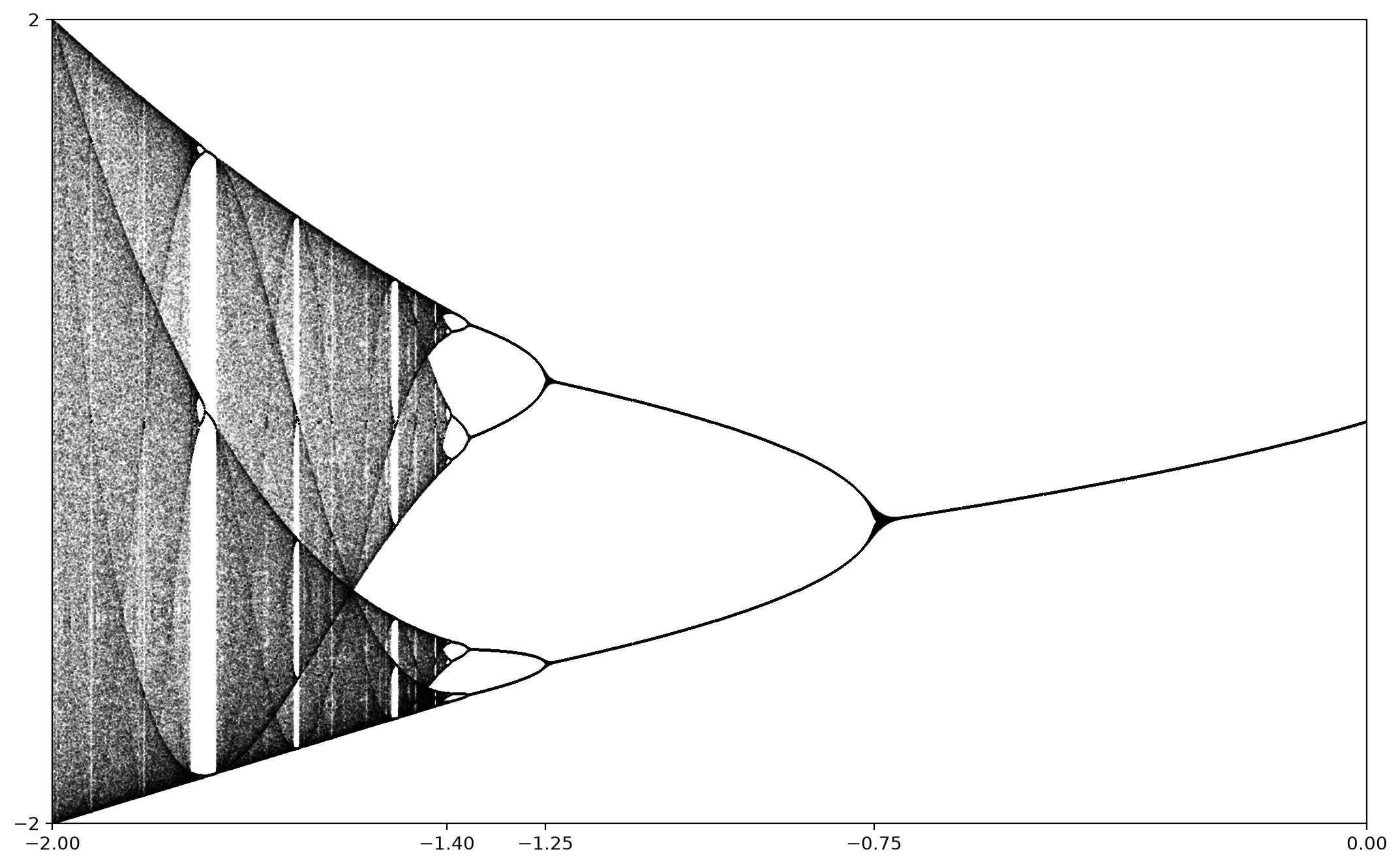
If we do this systematically for the quadratic family, plotting the columns to generate the bifurcation diagram, we get Figure 2.28
We can interpret this diagram as follows:
-
For \(-0.75 < c < 0\text{,}\) there is an attractive fixed point.
-
For \(-1.25 < c < -0.75\text{,}\) there is an attractive orbit of period \(2\text{.}\)
-
As \(c\) passes from just above \(-0.75\) to just below \(-0.75\text{,}\) the dynamics of \(f_c\) undergo a bifurcation.
-
For \(c\) just a little less than \(-1.25\text{,}\) there is an attractive orbit of period four. This orbit bifurcates soon into an attractive orbit of period 8. It appears that this behavior continues as \(c\) decreases.
-
For \(c\) somewhere around \(c\approx -1.4\text{,}\) the period doubling appears to stop and we get more complicated behavior.
Generally, a bifurcation occurs at a parameter value \(c=c_0\) if the global dynamical behavior of the function \(f_c\) undergoes some qualitative change as \(c\) passes through \(c_0\text{.}\) There are a number of different types of bifurcations that can occur, depending on the nature of the qualitative behavior under consideration. The bifurcations that are evident in Figure 2.28 in the range \(-1.4 < c < 0\) are called period doubling bifurcations.

