MML - Review for Exam 1
We will have our first exam Friday, Jan 31. This review sheet is now the final draft so most of the problems on that exam really should look a lot like something you see on this sheet.
Generally, I will expect solutions to the problems, as opposed to just answers. So, for example, if the answer to an optimization problem is \(y=5\), then the solution will consist of a clear explanation with correctly written supporting computations indicating why the answer is \(y=5\).
Note that there is a link at the bottom of this sheet labeled either “Start Discussion” or “Continue Discussion”, depending on the status of those discussions. Following that link will take you to my forum where you can create an account with your UNCA email address. You can ask questions and/or post responses and answers there.
The problems
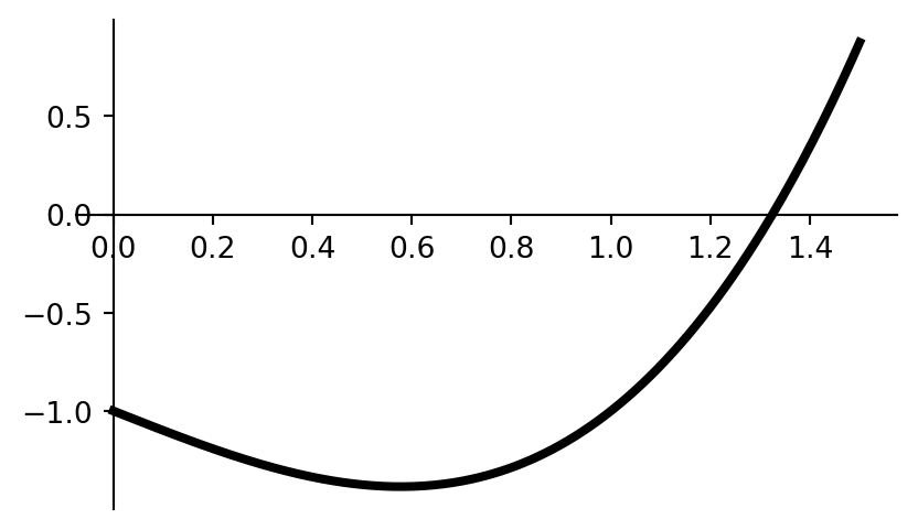
- The graph of the function \(f(x) = x^3 - x - 1\) over the interval \([0,1.5]\) is shown in figure 1.
- Find an equation of the line that’s tangent to the graph of \(f\) at the point where \(x=1\).
- Find the exact coordinates of the minimum shown in that graph.
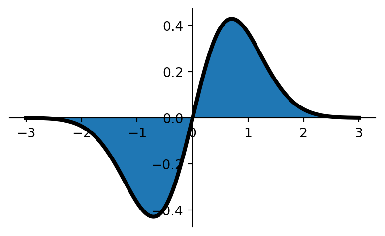
- The graph of \(f(x) = x\,e^{-x^2}\) over the interval \([-3,3]\) is shown in figure 2.
- What is the shaded area?
- What is the value of \[\int_{-3}^3 x\,e^{-x^2}\,dx?\]
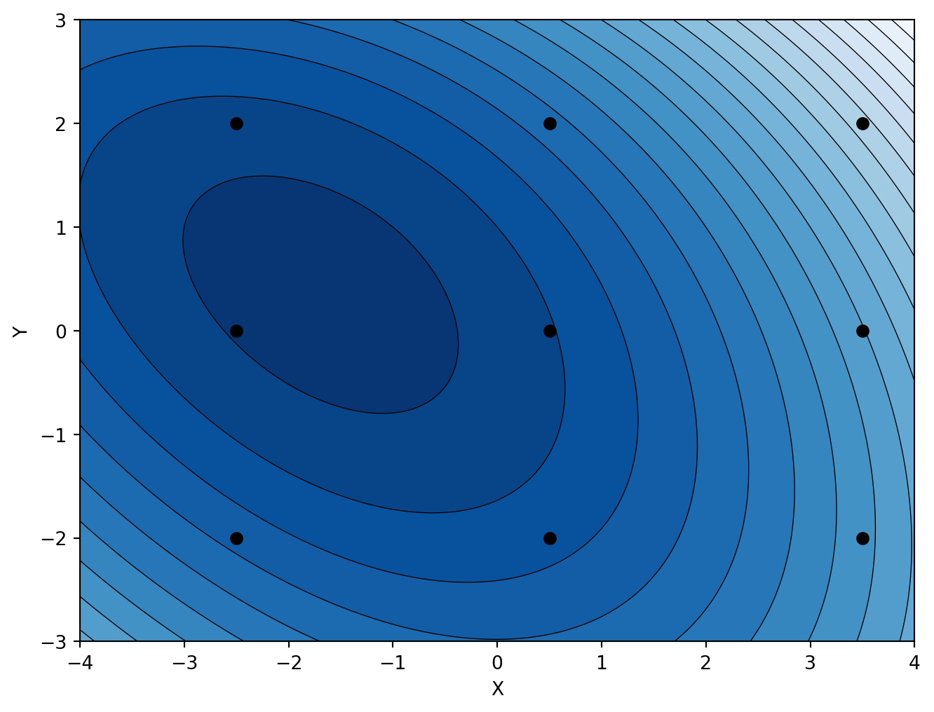
- Figure 3 shows a contour plot of \(f(x,y) = x^2+x y+3 x+y^2+2 y\).
- Identify any max, min, or saddle points that you see on the graph.
- Use the partial derivatives of \(f\) to find the exact locations of those points.
- Note the grid of 9 points on figure 3. For each of those points, draw the corresponding gradient vector emanating from that point. Be sure to pay careful attention to the direction and relative magnitude of those vectors.
- Suppose we wish to fit a least-squares regression line using a function of the form \(f(x) = ax+b\) to the data
[[0,0],[1,1],[2,1]]- Write down the function \(E(a,b)\) that expresses the total squared error of the approximation.
- Compute the two partial derivatives \(\partial E/\partial a\) and \(\partial E/\partial b\) of your error function.
- Set those partial derivatives each to zero and solve the resulting system.
- Interpret your solution to part (c) to obtain the least squares regression line.
- Provide examples of linear systems of three equations in three unknowns satisfying each of the following situations:
- The system has no solutions,
- The system has infinitely many solutions, and
- The system has exactly one solution.
- Let \(M\) denote the matrix \[
M = \begin{bmatrix}
2 & 1 & 5 & 10\\
1 & -3 & -1 & -2\\
4 & -2 & 6 & 12
\end{bmatrix}
\]
- Place \(M\) into reduced row echelon form.
- Assuming that \(M\) is an augmented matrix representing a \(3\times3\) system, use your reduced row echelon form to solve that system. If the solution set is infinite, you should parameterize that solution set.
- Write down a clear and complete statement of each of the following algebraic properties of the vector space \(\mathbb R^n\) and write down a componentwise proof of each of those laws.
- The commutative law of vector addition,
- The associative law of vector addition,
- The distributive law of scalar multiplication over vector addition.
- The matrix \(A\) and its reduced row echelon form \(R\) are shown below.
- Explain why you can tell immediately from \(R\) that \(A\) is a singular matrix.
- Use \(R\) to find a linear combination of the columns of \(A\) that sum to the zero vector in \(\mathbb R^4\).
\[A = \left[\begin{matrix}-2 & 0 & 2 & 4\\2 & -1 & -3 & -7\\-1 & -2 & -1 & -4\\1 & 1 & 0 & 1\end{matrix}\right]\]
\[R = \left[\begin{matrix}1 & 0 & -1 & -2\\0 & 1 & 1 & 3\\0 & 0 & 0 & 0\\0 & 0 & 0 & 0\end{matrix}\right]\]
Figures