Checkpoint 2.7.3
Find a value of \(c\) where \(f_c\) has a super-attractive orbit of period 5. Illustrate the resulting cobweb plot.
After the overall shape initiated by the period doubling cascade, the most conspicuous structure in the bifurcation diagram is probably the collection of vertical white strips. These correspond to regions where the \(c\) values lead to functions with attractive orbits. The largest such strip is called the period three window and a zoom into the period three window is shown in Figure 2.7.1.
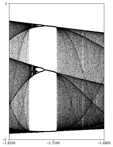
To understand the appearance of the period three window, we should plot the function \(f_c(x)=x^2+c\text{,}\) together with its third iterate, as well as with the line \(y=x\text{.}\) It looks like we should do so for several choices of \(c\) near \(c=-1.75\text{.}\) This is illustrated in Figure 2.7.2.

If we would like a more precise idea as to the location of the period 3 window, we can use our characterization of periodic oribts Definition 2.5.1. As \(c\) decreases through \(c\approx -1.75\) and beyond, there should be a value of \(c\) where \(f_c\) has a super-attractive orbit of period 3. By Corollary 2.5.3, this super-attractive orbit must contain the only critical point available, namely \(x=0\text{.}\) Thus, the value of \(c\) where this super-attractive orbit appears must satisfy the equation
This value of \(c\) should lie squarely in the period 3 window and is, in fact labeled in Figure 2.7.1. We can find a good numerical estimate with the following Sage code:
Find a value of \(c\) where \(f_c\) has a super-attractive orbit of period 5. Illustrate the resulting cobweb plot.