Theorem 2.6.2
If \(f:\mathbb C \to \mathbb C\) has an attractive or super-attractive orbit, then that orbit must attract at least one critical point.
A fabulous illustration of the types of behavior that can arise in a family of functions indexed by a single parameter and each with a single critical point can be generated as follows: For each value of the parameter, compute a large number points of the orbit of the critical point (maybe 1000 iterates). Since we're interested in long term behavior, rather than any transient behavior, discard the first few iterates (maybe 100). Then, plot the remaining points in a vertical column at the horizontal position indicated by the parameter.
The orbit of a critical point is called a critical orbit and its importance is due to the following theorem. If \(f:\mathbb C \to \mathbb C\) has an attractive or super-attractive orbit, then that orbit must attract at least one critical point.
Theorem 2.6.2
Regardless, the theorem has important implications for real iteration. For example, a polynomial of degree \(n\) can have at most \(n-1\) attractive orbits. Furthermore, if all the critical points happen to be real, we can find all the attractive behavior by simply iterating from the critical points. If we do this systematically for the quadratic family, plotting the columns to generate the bifurcation diagram, we get figure Figure 2.6.3
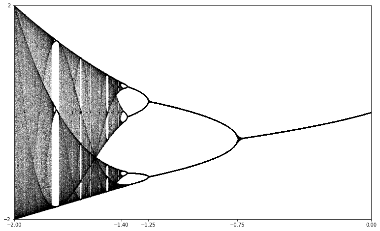
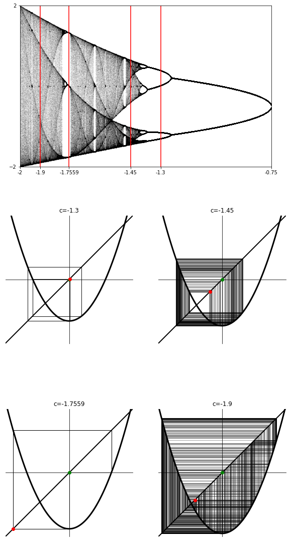
We can interpret this diagram as follows:
This interpretation is illustrated in Figure 2.6.4
Generally, a bifurcation occurs at a parameter value \(c=c_0\) if the global dynamical behavior of the function \(f_c\) undergoes some qualitative change as \(c\) passes through \(c_0\text{.}\) There are number of different types of bifurcations that can occur, depending on the nature of the qualitative behavior under consideration. The bifurcations that are evident in Figure 2.6.3 in the range \(-1.4 < c < 0\) are called period doubling bifurcations.