
Best Recent Content
-
Modeling 2D Heat Flow
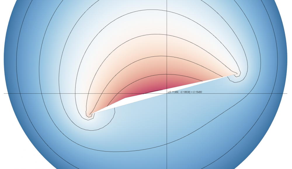
At $t=1s$, the temperature near the midpoint of the insulated edge of the triangle is approximately $.15480$.

-
Modeling a steady state heat distribution in 2D
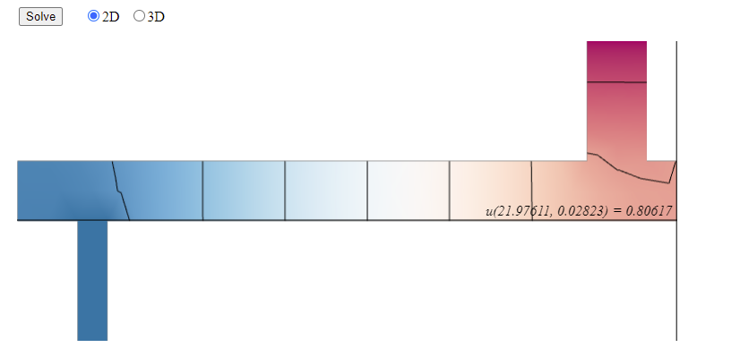
The temperature at the lower right corner is approximately 0.806 at a steady state.
-
Eigenranking
My matrix was:
matrix = [
[0,3,3,3,1],
[2,0,3,1,3],
[3,3,0,3,1],
[4,1,1,0,4],
[1,1,3,4,0]
]
and the eigen ranking was:
Team 3: rating = 0.4627375562956863
Team 1: rating = 0.46273755629568625
Team 4: rating = 0.46088857575916814
Team 5: rating = 0.4269598459305646
Team 2: rating = 0.4207551766581456
Team 3 is barely ahead of team 1 by rounding. But otherwise these two teams are dead even for the best team.
-
A radial heat flow problem
(1) We start by separating variables, and assume $u(r,t) = R(r)T(t)$. Our PDE then becomes
$$(RT)_t = (RT)_{rr} + \frac{1}{r}(RT)_r$$ or
$$RT' = R''T + \frac{1}{r}R'T.$$
Dividing both sides by $RT$, we get
$$\frac{T'}{T} = \frac{R''}{R} +\frac{1}{r}\frac{R'}{R} = -\lambda.$$
Thus, $\frac{T'}{T} = -\lambda$, so $T' = -\lambda T.$ Hence,
$$T = e^{-\lambda t}.$$ Meanwhile,
$$\frac{R''}{R} + \frac{1}{r}\frac{R'}{R} = -\lambda,$$ so
$$R'' + \frac{1}{r}R' = -\lambda R.$$
This can be rewritten as $$-(rR'(r))' = \lambda rR(r).$$
The solutions to this radial differential equation are the Bessel functions $$R(r) = c_1J_0\left(\sqrt{\lambda}r\right) + c_2Y_0\left(\sqrt{\lambda}r\right).$$
Since $Y_0$ is unbounded at $z=0, c_2$ must equal $0,$ so $$R(r) = c_1J_0\left(\sqrt{\lambda}r\right).$$
From our boundary conditions, we know $$R(1) = c_1J_0\left(\sqrt{\lambda}\right) = 0,$$ so
$$\sqrt{\lambda} = z_n, n=1,2,3...$$
where $z_n$ are the zeros of $J_0.$ Hence, the eigenvalues are $\lambda_n = z_n^2$ and the corresponding eigenfunctions are $R_n(r) = J_0(z_nr).$ Thus, our full solution is
$$u(r,t) = \sum_{n=1}^{\infty}c_ne^{-\lambda_n^2t}J_0(z_nr).$$
(2) By our initial conditions,
$$u(r,0) = \sum_{n=1}^{\infty}c_nJ_0(z_nr) = 5r^3(1-r).$$
Since Bessel functions satisfy the orthogonality condition,
$$c_n = \frac{\int_{0}^{1}5r^3(1-r)J_0(z_nr)rdr}{\int_{0}^{1}J_0^2(z_nr)^2rdr}.$$
Plugging an initial condition $u(r,0)$ into the "Radial heat flow" ObservableHQ page gives us the normalized Bessel function $F(r)$ for each term of the solution and its constant coefficient, which we'll denote $b_n,$ where
$$u(r,0) = \sum_{n=1}^{\infty}b_nF_n(r) = \sum_{n=1}^{\infty}b_n\frac{R_n(r)}{||R_n||}.$$
Since $u(r,0) = \sum_{n=1}^{\infty}c_nR_n(r),$ it follows that
$$c_n = \frac{b_n}{||R_n||}.$$
We plug in $u(r,0) = 5r^3(1-r)$ and find that
$$u(r,t) \approx \frac{0.17333401324973097}{0.3670927157694067}e^{-z_1^2t}J_0(z_1r) + \frac{-0.18156860394077448}{0.24060355211655088}e^{-z_2^2t}J_0(z_2r) + \frac{0.0731801393963544}{0.16437392311147672}e^{-z_3^2t}J_0(z_3r)$$
$$= 0.4721804759e^{-z_1^2t}J_0(z_1r) - 0.7546380855e^{-z_2^2t}J_0(z_2r) + 0.4452052857e^{-z_3^2t}J_0(z_3r)$$
(3)
Using the same Observable page, with N=10, we graph the function at time $t = 0.02$:
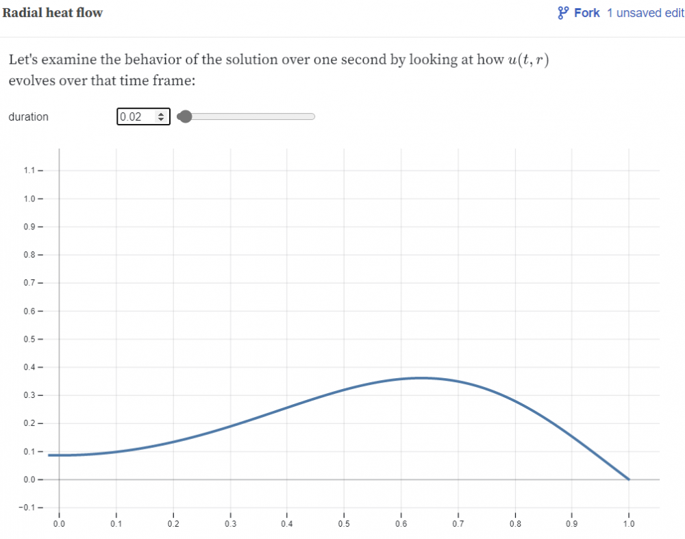
(4)
Using the final tool on the Observable page with $N=10$, we find $$u(0, 0.02) = 0.086.$$
-
Eigenranking
My matrix was matrix = [
[0,2,4,1,1],
[1,0,3,2,1],
[3,4,0,1,2],
[1,3,3,0,4],
[4,3,1,4,0]
]
The eigen ranking was:
Team 5: rating = 0.5351649756702808
Team 4: rating = 0.516996248452163
Team 3: rating = 0.43493231817629663
Team 1: rating = 0.3710347855055461
Team 2: rating = 0.3456593618764917
Team 5 was the best team.
-
Approximating an eigenfunction
I tried the following:
a = 0
b = 2
n =25
1) The 24x24 matrix that approximates the 2nd derivative is
$$U_{xx}=\begin{pmatrix} -312.5 & 156.25 & 0 & \ldots & 0 & 0 & 0\\ 156.25 & -312.5 & 156.25 & \ldots & 0 & 0 & 0\\ \ldots & \ldots & \ldots & \ldots & \ldots & \ldots & \ldots\\ 0 & 0 & 0 &\ldots & 156.25 & -312.5 & 156.25\\ 0 & 0 & 0 & \ldots & 0 & 156.25 & -312.5 \end{pmatrix}$$
2) The eigenvalue of smallest magnitude and its corresponding eigenvector are:
$$\lambda = -2.4642$$
$$\vec u = \begin{pmatrix} -0.0354\\ -0.0703\\-0.1041\\-0.1362\\-0.1662\\-0.1936\\-0.2179\\-0.2388\\-0.2559\\-0.2689\\-0.2778\\-0.2822\\-0.2822\\-0.2778\\-0.2689\\-0.2559\\-0.2388\\-0.2179\\-0.1936\\-0.1662\\-0.1362\\-0.1041\\-0.0703\\-0.0354\end{pmatrix}$$
3) The eigenfunction for this problem was: $$k* sin(\sqrt{-\lambda}*x)$$.
If we drop k, we get the following plot:
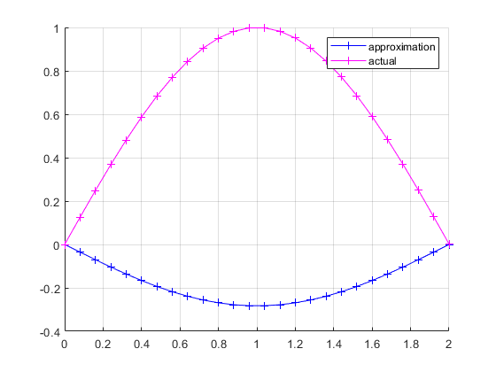
But if we let $k = -0.09\pi$, we get the following:
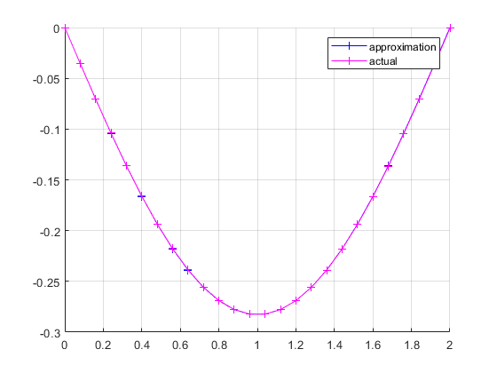
Now, I don't remember talking about using the approximation to find $k$ in class. @mark Could you explain why this was necessary here?
-
Eigenranking
My matrix was
matrix = [
[0, 4, 4, 4, 2],
[2, 0, 3, 4, 4],
[3, 1, 0, 3, 3],
[2, 1, 1, 0, 1],
[2, 3, 2, 2, 0]
]
The eigenranking was
Team 1: rating = 0.5676428888501164
Team 2: rating = 0.5140250259852949
Team 3: rating = 0.4266803335123048
Team 5: rating = 0.4096681506358447
Team 4: rating = 0.25234048971012685
And team 1 was the best.
-
Eigenranking
My Matrix was ;
matrix = [
[0,2,1,3,3],
[3,0,4,3,4],
[1,1,0,1,4],
[1,2,2,0,2],
[4,1,3,2,0]
]
Eigen Ranking ;
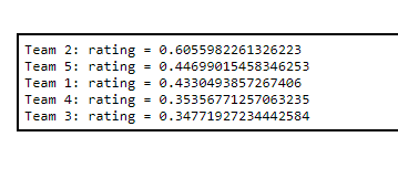
My best team being Team 2 by far.
-
Eigenranking
My matrix is
matrix = [
[0,1,3,2,4],
[2,0,2,2,2],
[3,1,0,1,3],
[4,4,3,0,3],
[2,4,4,4,0]
]
Team 5: rating = 0.5369571232846212
Team 4: rating = 0.5349109263288253
Team 1: rating = 0.4288594144453331
Team 3: rating = 0.35096444755792117
Team 2: rating = 0.34416697668415475
Team 5 was the best, followed very closely by team 4.
-
Eigenranking
My matrix:[
[0, 4, 2, 2, 1],
[1, 0, 4, 4, 1],
[1, 3, 0, 4, 4],
[1, 3, 2, 0, 1],
[2, 1, 4, 1, 0]
]
Team 3: rating = 0.5317387251068555
Team 2: rating = 0.4743664736534873
Team 1: rating = 0.43963279846587106
Team 5: rating = 0.41258201033241837
Team 4: rating = 0.3587888852214044
Clearly, team 3 has the advantage. However, since this is bling archery, you can never tell who will pull out on top.