

-
A radial heat flow problem
(1) We start by separating variables, and assume $u(r,t) = R(r)T(t)$. Our PDE then becomes
$$(RT)_t = (RT)_{rr} + \frac{1}{r}(RT)_r$$ or
$$RT' = R''T + \frac{1}{r}R'T.$$
Dividing both sides by $RT$, we get
$$\frac{T'}{T} = \frac{R''}{R} +\frac{1}{r}\frac{R'}{R} = -\lambda.$$
Thus, $\frac{T'}{T} = -\lambda$, so $T' = -\lambda T.$ Hence,
$$T = e^{-\lambda t}.$$ Meanwhile,
$$\frac{R''}{R} + \frac{1}{r}\frac{R'}{R} = -\lambda,$$ so
$$R'' + \frac{1}{r}R' = -\lambda R.$$
This can be rewritten as $$-(rR'(r))' = \lambda rR(r).$$
The solutions to this radial differential equation are the Bessel functions $$R(r) = c_1J_0\left(\sqrt{\lambda}r\right) + c_2Y_0\left(\sqrt{\lambda}r\right).$$
Since $Y_0$ is unbounded at $z=0, c_2$ must equal $0,$ so $$R(r) = c_1J_0\left(\sqrt{\lambda}r\right).$$
From our boundary conditions, we know $$R(1) = c_1J_0\left(\sqrt{\lambda}\right) = 0,$$ so
$$\sqrt{\lambda} = z_n, n=1,2,3...$$
where $z_n$ are the zeros of $J_0.$ Hence, the eigenvalues are $\lambda_n = z_n^2$ and the corresponding eigenfunctions are $R_n(r) = J_0(z_nr).$ Thus, our full solution is
$$u(r,t) = \sum_{n=1}^{\infty}c_ne^{-\lambda_n^2t}J_0(z_nr).$$
(2) By our initial conditions,
$$u(r,0) = \sum_{n=1}^{\infty}c_nJ_0(z_nr) = 5r^3(1-r).$$
Since Bessel functions satisfy the orthogonality condition,
$$c_n = \frac{\int_{0}^{1}5r^3(1-r)J_0(z_nr)rdr}{\int_{0}^{1}J_0^2(z_nr)^2rdr}.$$
Plugging an initial condition $u(r,0)$ into the "Radial heat flow" ObservableHQ page gives us the normalized Bessel function $F(r)$ for each term of the solution and its constant coefficient, which we'll denote $b_n,$ where
$$u(r,0) = \sum_{n=1}^{\infty}b_nF_n(r) = \sum_{n=1}^{\infty}b_n\frac{R_n(r)}{||R_n||}.$$
Since $u(r,0) = \sum_{n=1}^{\infty}c_nR_n(r),$ it follows that
$$c_n = \frac{b_n}{||R_n||}.$$
We plug in $u(r,0) = 5r^3(1-r)$ and find that
$$u(r,t) \approx \frac{0.17333401324973097}{0.3670927157694067}e^{-z_1^2t}J_0(z_1r) + \frac{-0.18156860394077448}{0.24060355211655088}e^{-z_2^2t}J_0(z_2r) + \frac{0.0731801393963544}{0.16437392311147672}e^{-z_3^2t}J_0(z_3r)$$
$$= 0.4721804759e^{-z_1^2t}J_0(z_1r) - 0.7546380855e^{-z_2^2t}J_0(z_2r) + 0.4452052857e^{-z_3^2t}J_0(z_3r)$$
(3)
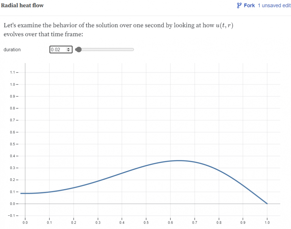
Using the same Observable page, with N=10, we graph the function at time $t = 0.02$:
(4)
Using the final tool on the Observable page with $N=10$, we find $$u(0, 0.02) = 0.086.$$

-
Eigenranking
My matrix was:
matrix = [
[0,1,4,3,3],
[2,0,2,4,3],
[3,3,0,3,2],
[2,1,1,0,2],
[3,1,3,1,0]
]
and my ranking was:
Team 3: rating = 0.5054388063612655
Team 1: rating = 0.5016207712530641
Team 2: rating = 0.48157957363128245
Team 5: rating = 0.4108981576640922
Team 4: rating = 0.30356553355238997
Team 3 was the best.
-
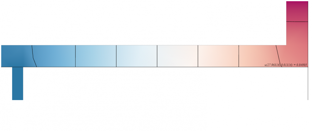
Modeling a steady state heat distribution in 2D
With $\kappa = 0$ and $f = 0$, the steady state temperature at the lower right corner of the bar is 0.84905.
-
Modeling 2D Heat Flow
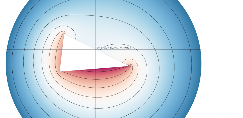
As can be observed in the screenshot above, the temperature near the midpoint of the insulated edge of the triangle (see my randomly generated problem for details of the model) is 1.04558.
-
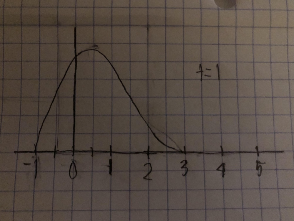
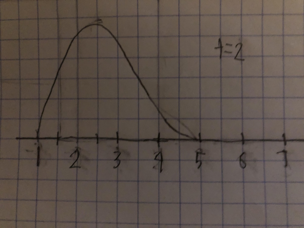
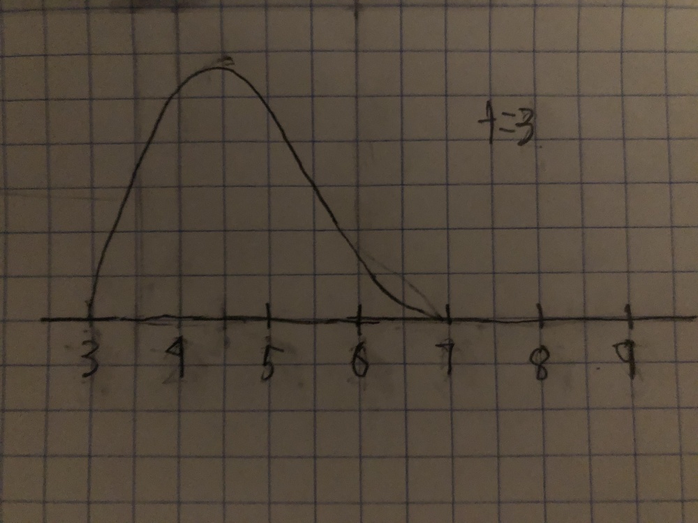
First order sketches
The solution to the PDE is
$$u = u_0(x - 2t),$$
so at each time interval, the graph above will shift to the right by two units. Here are sketches of the graph at each of the three times:
If we changed the PDE to $u_t + 2u_x = -u$, the solution becomes
$$u = u_0(x - 2t)e^{-t},$$
so $u$ will decay over time, approaching zero at large values of $t$.
