Map Projection
An Intro for Multivariable Calculus
Abstract
This document provides an introduction to map projections for students of multivariable calculus. The emphasis is on distortion of area and angles of cylindrical projections with a particular objective of understanding Mercator’s projection.
Introduction
In multivariable calculus, we study higher dimensional calculus, that is, derivatives and integrals applied to functions mapping \(\mathbb{R}^m\) to \(\mathbb{R}^n\). Viewed in this context, the study of map projection is quite natural since we are mapping the surface of a globe to a planar rectangle. The globe is naturally parameterized in terms of two variables, latitude \(\varphi\) and longitude \(\theta\). Thus, we could think of a map projection as a function \[T:\mathbb{R}^2 \to \mathbb{R}^2 \text{ or } T(\varphi,\theta) = (x(\varphi,\theta), y(\varphi,\theta)).\] Isn’t that exactly the kind of thing we study in Calc III???
Example map projections
The earth, as we well know, is approximately spherical; it is best represented as a globe. For convenience both physical and conceptual, however, we frequently represent the spherical earth with a flat map. Such a representation must involve distortion. The process is illustrated in Figure 1.
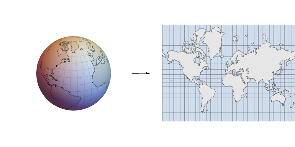
The projection shown in Figure 1 is called Mercator’s projection. Mercator created his projection in 1569. Although it was not universally adopted immediately, it represented a major breakthrough in navigation because paths of constant compass bearing are represented as straight lines. Ultimately, this property follows from the fact that Mercator’s projection is a cylindrical, conformal projection. A major goal of this document is to understand these facts.
We will not really fully understand a map projection until we know and understand the formula defining the projection. We’ll get to that formula for Mercator’s projection by the time this document is done (which it isn’t, just yet).
Of course, there are a huge number of map projections. The interactive image below shows just a few.
Two big questions
When choosing a map projection there are two big questions that we should ask about the map.
First, what properties should the map have? Should it represent equal areas in equal proportions? Should it properly represent distance to some central point? Will it represent direction in some canonical way?
Second, what type of map projection is it? Was it constructed by projection onto a cylinder, plane, or cone? A proper understanding of map type helps us analyze the first question.
Properties of maps
When considering what map projection to use for a particular purpose, you need to know what properties the map should have. There are many properties that might be relevant to all sorts of questions but there are two major properties that we will consider here.
Equal area maps
Does the map need to be equal area (also called area preserving)? This means quite simply that areas are represented in their correct proportions. Mercator’s projection is not equal area. Greenland (with an area of about \(2.2\) million square kilometers) looks larger than South America (with an area of about \(17.8\) million square kilometers). The Equal Earth, shown on the right in Figure 2, is an equal area map.
Why equal area?
Some maps are designed to illustrate some simple concept, such as population, political affiliation, region or whatever. In this case, it’s common to strip out most unnecessary details to focus on the issue at hand. This type of map is commonly called a thematic map or choropleth.
When designing a choropleth, it’s often desirable for the map to be equal area, particularly when the shading is intended to indicate density. The reason is pretty clear, I suppose. If you shade a Mercator map by temperature, for example, then your impression of average temperature is likely to be skewed towards the cooler side due to the tremendous inflation near the poles.
The map in Figure 3 shows a choropleth for population density in the contiguous US.
Conformal maps
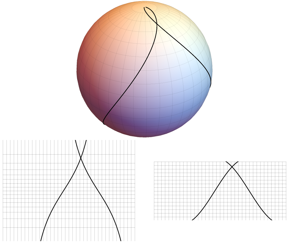
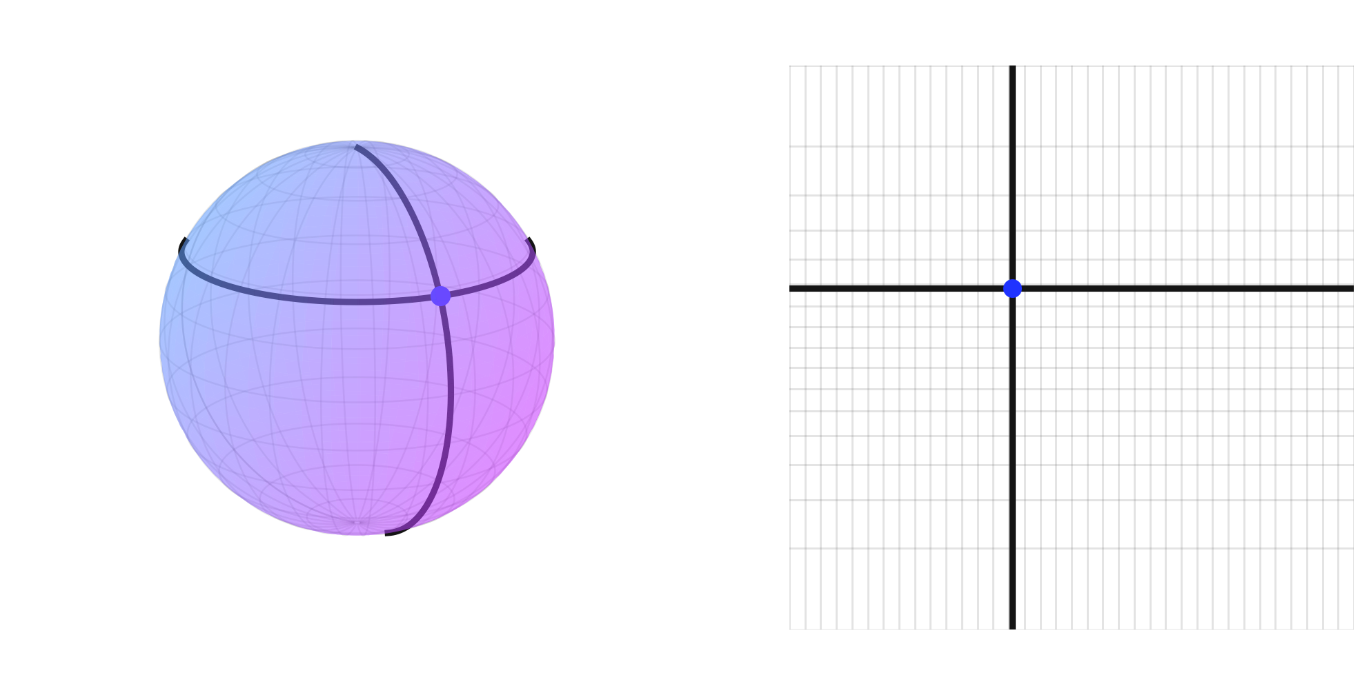
Should the map be conformal? This means that the map preserves angles. To understand this, suppose we have two paths on a globe that intersect at some angle. If we take the image of these paths under a conformal transformation, the angle will be the same. This is illustrated in Figure 4, where we see the image of two paths on the globe under Mercator’s projection and the equi-rectangular projection. The angle is preserved under Mercator’s projection but not under the equi-rectangular projection.
Why conformal???
When navigating from one spot to another, it’s often desirable to have a conformal map. We’ll talk more about this when we discuss Mercator’s map in more detail
Balancing objectives
Since this is a math class, let’s state a couple of theorems:
This seems reasonably easy to believe. To be distance preserving in this fashion, the projection would have to preserve shapes exactly and, in particular, it would preserve any curvature inherent in the shape. Thus, we can’t flatten a curved surface without distorting some distances. Nonetheless, we can often do a reasonable job of minimizing that distortion, particularly on maps of small regions. That’s obviously a desirable for maps designed for navigation.
Our second theorem is a little more challenging:
This is a well-known and long established theorem that’s been proven mathematically; it is not a topic of discussion. Both properties are desirable in certain situations, though, so it’s essential to know when to design your map with the appropriate property. Here are some criteria to consider when choosing between these properties:
Centered equidistant maps
While we can’t represent all distances on a map in their correct proportion, we can sometimes represent some collection of distances correctly. Such a map is called an azimuthal equidistant map. Figure 5 shows circles centered at Asheville in two different projections. In only one of those directions do the circles look like circles, though!
Types of map projections
When we refer to the type of a map projection we are essentially classifying the projections roughly by the way they are constructed. These generally fall into one of three types: - Cylindrical, - Conic, or - Azimuthal.
There are variations on these themes, such as composite maps formed by combining other maps and interrupted maps with discontinuities. We’ll focus on the three main types here, though.
Cylindrical projections
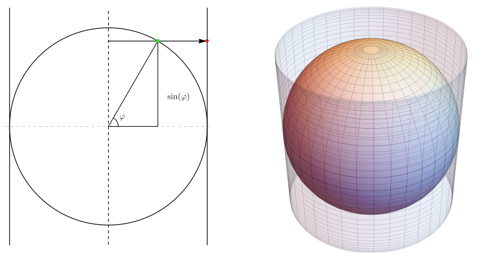
Conceptually, a cylindrical projection can be visualized by wrapping a cylinder around a globe and projecting points on the globe out to the cylinder. Lambert’s equal area projection is obtained quite literally from a geometric projection where each point on the globe is projected out radially from a line that goes through the North and South poles. This is illustrated in Figure 6.
When we refer to a “cylindrical projection”, we don’t mean that it arises as a literal geometric projection in the sense that Lambert’s does. Rather, we mean that the parallels all appear on the map as horizontal lines of constant width and that the meridians are evenly spaced and are perpendicular to the parallels. This geometric characterization leads to an algebraic form that a cylindrical projection must have, namely: \[T(\varphi,\theta) = (\theta,h(\varphi)).\] We have several examples of this by now:
- The equirectangular projection: \(T(\varphi,\theta) = (\theta,\varphi)\),
- Lambert’s equal area projection: \(T(\varphi,\theta) = (\theta,\sin(\varphi))\), and
- Mercator’s projection: \(T(\varphi,\theta) = (\theta, \ln(|\sec(\varphi) + \tan(\varphi)|))\).
Of these, only Lambert’s is a literal projection. Nonetheless, all cylindrical projections share similarities and can be analyzed in similar ways.
Azimuthal projections
Azimuthal is just a groovy word meaning planar. Conceptually, a polar, azimuthal projection can be visualized by placing a plane tangent to the globe at one pole and projecting the sphere onto this plane.
There are multiple ways this projection process could go. Two possibilities called the stereograph and the orthographic projections are shown in Figure 7.
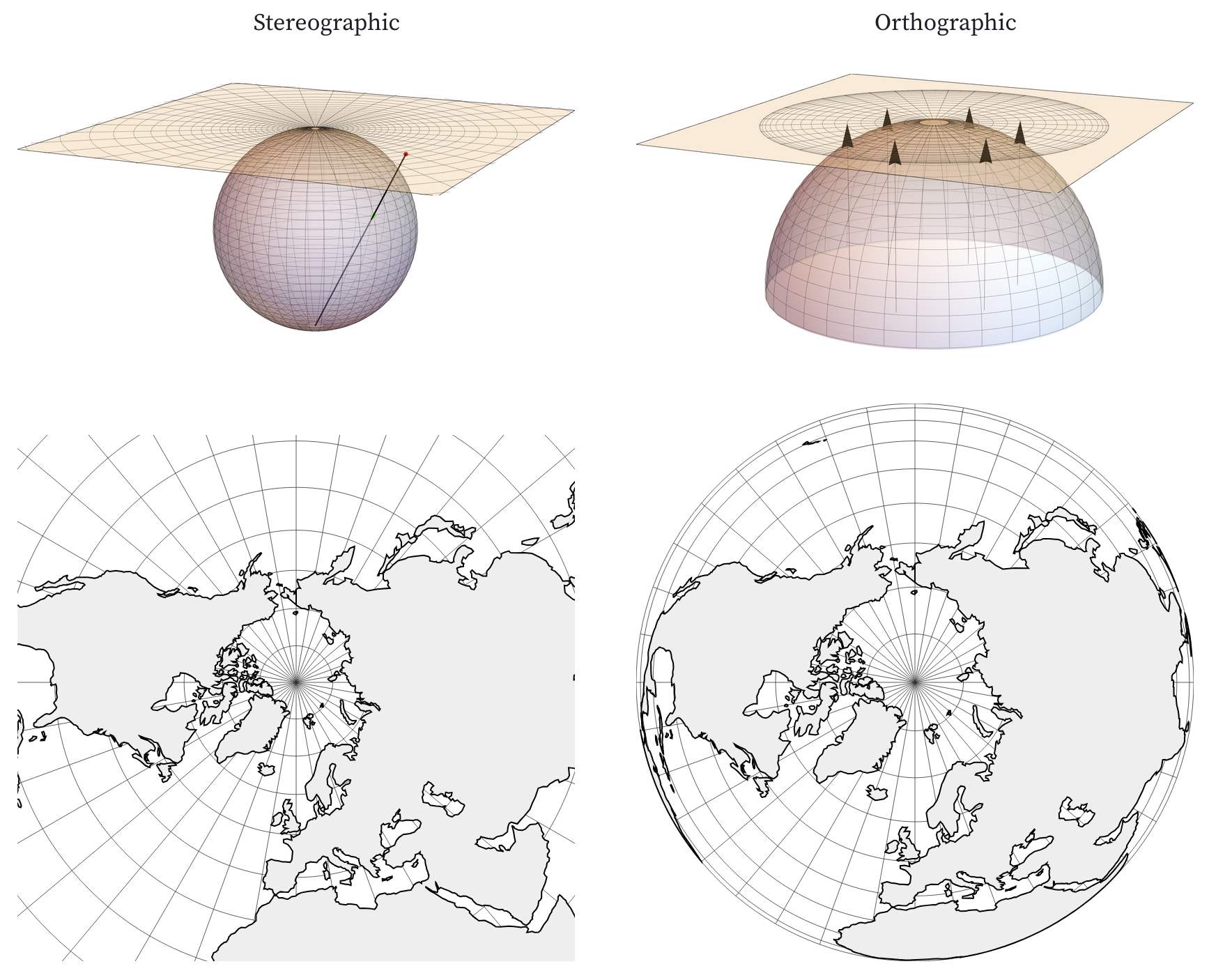
The stereographic projection is conformal while the orthographic is neither conformal nor equal area. Both distort distance quite a lot as we move away from the pole.
All polar azimuthal projections map parallels to concentric circles centered at the point of tangency with the meridians appearing as equally spaced rays emanating from the center. This implies that the general form of a polar azimuthal projection should be \[T(\varphi,\theta) = (r(\varphi)\cos(\theta), r(\varphi)\sin(\theta)).\] Put another way, we simply need to know how to space out the circles representing the parallels as we move away from the center and the function \(r(\varphi)\) tells us exactly how to do so.
More generally, any function \(T(\varphi,\theta)\) of this form is considered to be a polar azimuthal projection; it needn’t arise from an actual physical process. An important example is the azimuthal equidistant projection where \(r(\varphi)\) is defined to be proportional to the actual distance along the globe from the pole to any point at latitude \(\varphi\). This map has the property that distances from any point to the pole are represented proportionally, as in Figure 8.
Of course, an azimuthal map can be centered at any point, like our Asheville equidistant map shown in Figure 5.
Conic projections
Conceptually, a conic projection is obtained by projecting a sphere onto a cone and then cutting the cone so that it lies flat on a plane, as shown in Figure 9.

If the cone is tangent to the sphere, there will be one standard parallel along which there is no distortion of length. More often, the cone intersects the sphere along two parallels, which become standard parallels on the map. As a result, conic projections can achieve very small distortion along a large area in a temperate zone.
Like azimuthal projections, the parallels of a conic projection map to circular arcs and the meridians map to rays emanating from the common center of those circles. Unlike an azimuthal projection, the common center of the circles typically lies off the map.
Conic projections are not generally appropriate for whole earth maps. They do a great job representing large regions restricted to the temperate zones, though. One nice example of this is the official state map of North Carolina!
Map analysis
We now turn to the central question of how we analyze a map to determine what properties it might have. More specifically, what will make a map conformal or equal area.
Scale factors
If we move from point \(A\) to point \(B\) on the globe, this induces a change of distance on the map. The corresponding scaling factor is simply the change in distance on the globe divided by the change in distance on the map. This simple idea is the key to understanding which geometrical properties are preserved by a map projection.
To see why scale factors are so important to the understanding of geometric properties of transformations, we’ll focus on some particularly simple examples—namely, the transformation of rectangles in the plane. In spite of the level of simplicity, the ideas generalize quite readily to our setting.
Suppose we want our transformation to be conformal, i.e., it should preserve angles. In particular, if we draw a rectangle in the plane, the angle that the diagonal of the rectangle makes with either side should be preserved under the transformation. This situation is illustrated in Figure 11, where it becomes almost immediately apparent what property the transformation should have.
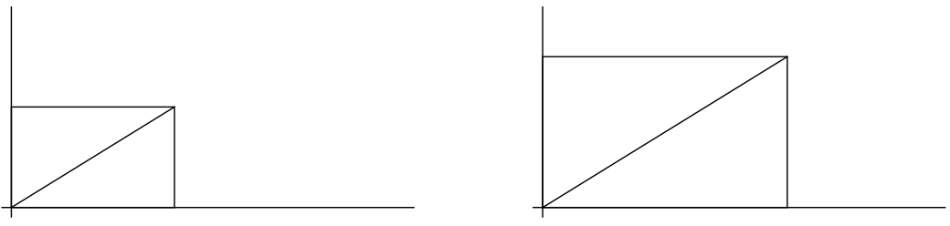
This statement indicates that the equality of scaling factors is a necessary condition. It can be proved that it is also a sufficient condition. That is, if the transformation scales by the same amount in both the horizontal and vertical directions, then it will be conformal.
Now, suppose that we’d like our transformation to preserve area. The transformation in Figure 11 clearly does not preserve area, but the transformation in Figure 11 does. Again, the figure indicates how to obtain the desired property. If we scale by the factor \(M\) in one direction, we’ve got to scale by the factor \(1/M\) in the other.
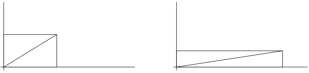
This condition is again sufficient as well as necessary.
Scale factors for a cylindrical projection
When we apply these ideas to a cylindrical map projection (which of course maps a globe to a plane), we take the scale factors along a parallel and along a meridian to be the two cardinal directions. We denote these scaling factors by \(M_{\varphi}\) and \(M_{\theta}\), respectively.
Thus, if we are at the point \((\varphi, \theta)\) on the globe, our cylindrical map projection will be conformal near that point if \(M_{\varphi} = M_{\theta}\) there. A cylindrical map projection will be area preserving if \(M_{\varphi} = \frac{1}{M_{\theta}}\) there.
Suppose a point on the globe is at position \((\varphi, \theta)\). Consider the parallel through that point. On the globe, that parallel is a circle of radius \(\cos(\varphi)\). (Take another look at ?@fig-geometricLambert to convince yourself of this.) Thus, the circumference of that parallel on the globe is \(2\pi \cos(\varphi)\).
Furthermore, this parallel maps to a line segment that stretches the whole width of the map, as shown in Figure 13. The length of that segment is \(2\pi\). Thus the scaling factor along the parallel is a uniform
\[ M_{\varphi} = \frac{2\pi}{2\pi \cos(\varphi)} = \sec(\varphi). \]
Analysis of the scaling factor along a meridian is a little trickier. Recall that our cylindrical projection has the form \(T(\varphi, \theta) = (\theta, h(\varphi))\). While \(M_{\varphi}\) is uniform and depends only on \(\varphi\), \(M_{\theta}\) is not necessarily uniform and depends on the function \(h\).
Here is the key observation. Suppose we are at a point with latitude \(\varphi\) and we increase the latitude a bit to \(\varphi + t\). On the globe, we move a distance \(t\). (This follows from the definition of radian measure.) On the map we move from the point \(h(\varphi)\) to \(h(\varphi + t)\). Thus our scaling factor (the change of distance on the map over the change in distance on the globe) is
\[ \frac{h(\varphi + t) - h(\varphi)}{t}. \]
Of course, we are interested in the local scaling factor. Thus we take a limit as \(t \to 0\) to obtain \(h'(\varphi)\).
This pair of scaling factors is worth knowing. For a cylindrical map projection \(T(\varphi, \theta) = (\theta, h(\varphi))\),
- the scaling factor \(M_{\varphi}\) along a parallel is \(\sec(\varphi)\), and
- the scaling factor \(M_{\theta}\) along a meridian is \(h'(\varphi)\).
Application
We are now in a position to understand why Lambert’s map in ?@fig-equiAndLambert is equal area and why Mercator’s map in Figure 1 is conformal. In fact, the analysis is quite easy for both.
Lambert’s equal area map
Recall that the formula is \(T(\varphi, \theta) = (\theta, \sin(\varphi))\). Thus, \(M_{\theta} = \cos(\varphi)\) and \(M_{\varphi} = \sec(\varphi)\). Since these are reciprocals, the projection is equal area. That’s it!
Mercator’s projection
Let us now put ourselves in Mercator’s shoes and ask, what function \(h(\varphi)\) will force the cylindrical projection \(T(\varphi, \theta) = (\theta, h(\varphi))\) to be conformal?
Well, we need \(h'(\varphi) = \sec(\varphi)\). Thus, we should take
\[ h(\varphi) = \int_0^{\varphi} \sec(\phi)\, d\phi = \ln\left| \sec(\varphi) + \tan(\varphi) \right|. \]
There you are!
Final comments
Why map projections??
Why should we study map projections in a class like Calc III?
Map projections are literally functions that map the two dimensional surface of a sphere to a planar, two dimensional region. We can analyze the fundamental questions of shape and area distortion using derivatives and express some map projections as integrals. This all fits squarely in the realm of multidimensional calculus!
It’s also a beautiful visual topic with a rich history an all sorts of interesting little fact nuggets. Furthermore, the ability to interpret maps (from specialized local maps to global maps illustrating geopolitics) is an important skill. That’s why several majors at UNCA, like ATMS and ENVR, have their own GIS courses. Some larger schools have GIS courses within other departments like political science or history.
So, it’s a really great topic and nice fit for a math course at a liberal arts school!
The Peters world map controversy
The Gall-Peters projection was first described in 1855 by the Scot James Gall and rediscovered in the 1960s by the German Arno Peters. In the 1970s, Peters vigorously promoted his map as superior to the Mercator map projection, essentially since it’s equal area. Peters was dismissed as a bit of crank by cartographers of the time and the whole affair become known as the Peters world map controversy. You can see this parodied in The West Wing.
To be clear, Mercator’s map is probably not ideal for a classroom wall map and the Gall-Peters map is a reasonable alternative. It seems that Peters’ “mistake” was his failure to realize
- that Mercator had a different objective and
- there are many area preserving maps.
One widely used equal earth map projection today is the equal earth projection. You can read about its motivation in this presentation.
Problems
The equi-rectangular projection is the cylindrical projection defined by \(T(\varphi ,\theta )=(\theta ,\varphi )\). Compute the general distortion factors \(M_p\) and \(M_m\) for \(T\) as functions of \(\varphi\) and \(\theta\). Use this to explain why the equi-rectangular projection is neither conformal nor equal area.
Mercator’s projection is the cylindrical projection defined by \(T(\varphi ,\theta )=(\theta ,\ln (|\sec (\varphi )+\tan (\varphi )|))\). Compute the general distortion factors \(M_p\) and \(M_m\) for \(T\) as functions of \(\varphi\) and \(\theta\). Use this to prove that Mercator’s projection is conformal.
Lambert’s equal area, cylindrical projection is the cylindrical projection defined by \(T(\varphi ,\theta )=(\theta ,\sin (\varphi ))\). Compute the general distortion factors \(M_p\) and \(M_m\) for \(T\) as functions of \(\varphi\) and \(\theta\). Use this to prove that Lambert’s projection is equal area.
Use Figure 2 to explain why the Equal Earth projection is not conformal.
Compute the scaling factors \(M_{\varphi }\) and \(M_{\theta }\) here in Asheville for both Mercator’s projection and the equi-rectangular projection. How close is the equi-rectangular projection to being conformal here? How close is Mercator’s projection to being area preserving here?
New York and Barcelona lie very close to the same latitude having the coordinates: \(74^{\circ}W\) by \(41^{\circ}N\) and \(2^{\circ}E\) by \(41^{\circ}N\).
- On a cylindrical or psuedo-cylindrical maps, the naive `straight line’ between Barcelona and New York lies on the common parallel. What is the distance between the two cities along this parallel?
- What is the actual shortest distance between those two cities?
Hint: Note that both curves are parts of circles.