LLM tokenization visualization
One simple way (maybe, too simple?) to think of an LLM is as a next token predictor. Given a sequence of tokens (each of which often corresponds to a word or part of a word), an LLM predicts several next most likely tokens and chooses one. That new sequence of tokens is fed back in and the process iterates.
This tool allows you to visualize one step of this process by taking input text and
- Breaking it into tokens and
- Listing the 10 most likely next tokens according to one LLM.
The visualizer
Enter some text and hit the “Tokenate it!” button to see token chunks and possible completions.
Tokenization
Next token candidates
| Rank | Continuation | Probability |
|---|---|---|
Implementation details
The tokenizer uses js-tiktoken - a fast, open source tokenizer that uses byte pair encoding.
The next token predictions are obtained from Google’s Gemma 4 26B A4B, a 26 billion parameter model with about 4 billion active parameters per token. This model is open source and provides logprobs and top_logprobs, which are essential for this demo.
Gemma probably uses somewhat different tokens than those produced by js-tiktoken. This page is meant to provide an educational illustration of a couple important LLM concepts, though. The tokenizer and predictor are chosen more for convenience than perfection.
Some mathematical comments
Today’s large language models are effectively very large neural networks with specialized architecture. An example of a much simpler neural network is illustrated below.
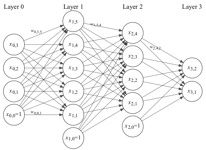
Each \(x_{0,i}\) on the left represents an input and each \(x_{3,j}\) on the right represents an output. In the context of a large language model, the input nodes might represent a sequence of input tokens (represented as numerical vectors) and the output nodes might correspond to potential next tokens. The idea is to assign a numerical probability to each potential output.
Once we’ve assigned an input, that input propagates from left to right through the network via a formula that looks like
\[x_{i,k} = g_i\left(\sum_{j=0}^{n_{i-1}} w_{i-1,j,k} \times x_{i-1,j}\right).\]
Each \(w_{i-1,j,k}\) is called a weight or parameter and associated with an edge; a few edges are labeled with their weights in the diagram. The \(g_i\) is called an activation. In the context of a predictor, the last activation translates numerical scores to probabilities using a formula like so:
\[P_k = g_i(z_k) = \frac{e^{z_k}}{\sum_j e^{z_j}}.\]
Of course, an LLM is much larger. The neural network illustrated above has 54 edges and, therefore, 54 parameters. Gemma 4 26B A4B has 26 billion parameters. It also has a more complicated architecture. Nonetheless, many of the fundamental ideas are the same.