d = [2.57,4.43,2.09,7.68,4.77,2.12,5.13,5.71,5.33,3.31,7.49,4.91,2.58,1.08,6.60,3.91,3.97,6.18,5.90]
While it might be important for researchers to assess the threat of mercury in the ocean, they do not want to go kill more dolphins to get that data. What can they conclude from this data set, even though it's a bit too small to use a normal distribution?
The basics
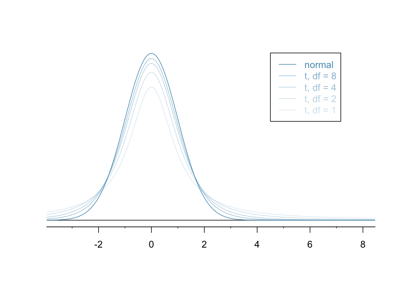
The normal distribution, as awesome as it is, requires that we work with large sample sizes - at least 30 and more is better.
The $t$-distribution is similar but better suited to small sample sizes.
Just as with the normal distribution, there's not just one $t$-distribution but, rather, a family of distributions.
Just as there's a formula for the normal distribution, there's a formula for the $t$-distribution. It's a bit more complicated, though: $$ f(t) = \frac{\left(\frac{\nu-1}{2}\right)!} {\sqrt{\nu\pi}\,\left(\frac{\nu-2}{2}\right)!} \left(1+\frac{t^2}{\nu} \right)^{\!-\frac{\nu+1}{2}} $$ The parameter $\nu$ is an integer representing the degrees of freedom which is the sample size minus one.
Like all continuous distributions, we compute probabilities with the $t$-distribution by computing the area under a curve. We do so using either a computer or a table.
The mean of the $t$-distribution is zero and its variance is related to the degrees of freedom $\nu$ by $$\sigma^2 = \frac{\nu}{\nu-2}.$$
Unlike the normal distribution, there's no easy way to translate from a $t$-distribution with one standard deviation to another standard one. As a result, it's less common to use tables and more common to use software than it is with the normal.
Given a particular number of degrees of freedom, however, there is a standard way to derive a $t$-score that's analogous to the $z$-score for the normal distribution. This $t$-score is a crucial thing that you need to know when using tables for the $t$-distribution.
Finding the confidence interval
Finding a confidence interval using a $t$-distribution is a lot like finding one using the normal. It'll have the form $$ [\overline{x}-ME, \overline{x}+ME], $$ where the margin of error $ME$ is $$ ME = t^* \frac{\sigma}{\sqrt{n}}. $$
Here's how we would use Python to compute the mean and standard deviation for the dolphin problem:
import numpy as np
m = np.mean(d)
s = np.std(d, ddof=1)
[m,s]
The crazy looking ddof parameter forces np.std to compute the sample standard deviation, rather than the population standard deviation - i.e. it uses an $n-1$ in the denominator, rather than an $n$.
Next, the multiplier $t^*$ can be computed using t.ppf from the scipy.stats module:
from scipy.stats import t
tt = t.ppf(0.975,df=18)
tt
Note that the $t^*>2$ and $2$, of course, would be the multiplier for the normal distribution. This makes some sense because the $t$-distribution is more spread out than the normal. From here, our confidence interval is:
[m-tt*s/np.sqrt(19), m+tt*s/np.sqrt(19)]
Using a table
Note that we can also find that $t^*=2.1$ in the $t$-table on our webpage, where we see something that looks like so:
| one tail | 0.100 | 0.050 | 0.025 | 0.010 | 0.005 |
| two tails | 0.200 | 0.100 | 0.050 | 0.020 | 0.010 |
| df 1 | 3.08 | 6.31 | 12.71 | 31.82 | 63.66 |
| 2 | 1.89 | 2.92 | 4.30 | 6.96 | 9.92 |
| ... | ... | ... | ... | ... | ... |
| 18 | 1.33 | 1.73 | 2.10 | 2.55 | 2.88 |
The entries in this table are called critical $t^*$ values. The columns indicate several common choices for confidence level and are alternately labeled either one-sided or two. The rows correspond to degrees of freedom. Now, look in the row where $df=18$ and where the two-sided test is equal to 0.05. we see that $t^*=2.1$.
A hypothesis test
We can also use the $t$-distribution to do hypothesis tests with small sample size. When running a hypothesis test for the mean of numerical data, we have a hypothesis test that looks like so:
\begin{align} H_0 : \mu=\mu_0 \\ H_A : \mu\neq\mu_0. \end{align}In this notation, $\mu$ denotes the actual population mean and $\mu_0$ is an assumed, specific value. The question is, whether recently collected data supports the alternative hypothesis (two-sided here, though it could be one-sided).
As before, we compute something that looks like a $Z$-score, though more generally, it's typically called a test statistic. Assuming the data has sample size $n$, mean $\bar{x}$, and standard deviation $s$, then the test-statistic is $$\frac{\bar{x}-\mu_0}{s/\sqrt{n}}.$$ We then compare the test statistic to the appropriate $t$-table to determine whether to reject the null hypothesis or not.
Example
Returning to the dolphin example, let's suppose that the desired average level of mercury is 3. Let's run a hypothesis test to see if the data supports the alternative hypothesis that the actual average is larger than $3$ to a 99% level of confidence. Recall that the computed mean and standard deviation are $$\bar{x} = 4.51368 \text{ and } s = 1.830479.$$ Also, the sample size is 19 so our test statistic is $$\frac{4.51368-3}{1.830479/\sqrt{19}} \approx 3.604509.$$ Referring to the CDF for the $t$-distribution with 18 degrees of freedom, we find the following $p$-value:
t.cdf(-3.604509,18)
Thus, we reject the null!
We could also note that our test statistic is outside our rejection point of about $2.55$ we can see that in the table above or by the following computation:
t.ppf(0.01,18)
The $t$-distribution and sample proportions
We can apply the $t$-distribution to either a sample mean for numerical data or a sample proportion for categorical data - just as we would use the normal distribution when the sample size is large enough.
Example
Conventional wisdom states that about 5\% of the general population has blue eyes. Scanning our class data, I find that 2 out of the 10 of us, or 20\%, has blue eyes. Should this evidence dissuade us from believing the generally accepted value?
More precisely, if $p$ represents the proportion of folks with blue eyes, we are considering the hypothesis test:
\begin{align} H_0 &: p=0.05 \\ H_A &: p\neq0.05. \end{align}We would compute a test statistic in exactly the same way that we compute a $Z$-score:
$$\frac{\hat{p}-p}{\sqrt{p(1-p)/n}} = \frac{0.2-0.05}{\sqrt{0.05\times0.95/10}} \approx -2.176$$This is clearly past the 95\% cuttoff, if we were using a normal distribution. If we look up the 95\% cuttoff for the $t$-distribution with 9 degrees of freedom in our table, however, we find a cuttoff of 2.26. Thus, we fail to reject the null.