Probability theory
Probability theory is the mathematical foundation for statistics. It's covered in chapter 2 of our text. In this portion of our outline, we'll look briefly at the beginning of chapter 2.
What is probability?
- A random event is an event where we know which possible outcomes can occur but we don't know which specific outcome will occur.
- The set of all the possible outcomes is called the sample space.
- If we observe a large number of independent repetitions of a random event, then the proportion $\hat{p}$ of occurrences with a particular outcome converges to the probability $p$ of that outcome.
That last bullet point is called the Law of Large Numbers and is a pillar of probability theory. It can be written symbolically as
$$P(A) \approx \frac{\# \text{ of occurrences of } A}{\# \text{ of trials}}.$$More importantly, the error in the approximation approaches zero as the number of trials approaches $\infty$.
Again, this is a symbolic representation where:
- The symbol $A$ represents a set of possible outcome contained in the sample space. Such a set is often called an event.
- The symbol $P$ represents a function that computes probability.
- Thus, $P(A)$ tells us the probability that the event $A$ occurs.
In an experimental context, the Law of Large Numbers can be used to compute the probability of an event. We can illustrate this process with a computer experiment!
# Load some standard libraries
%matplotlib inline
import matplotlib.pyplot as plt
import numpy as np

# A couple of functions for random number generation
from numpy.random import choice, seed

# seed the random number generator for reproducibility
# seed(2)

# Number of flips
n=100

# Probability of a head on each flip
p = 0.6

# Generate the flips - 0 or 1 for tail or head.
flips = choice([0.0,1.0], size=n, p=[1-p,p])

# Generate the cumulative sums,
# i.e. [1,0,1,0,0,1] -> [1,1,2,2,2,3]
sums = np.cumsum(flips)

# Convert sums to proportions
# i.e. [1,1,2,2,2,3] -> [1,1/2,2/3,1/2,2/5,1/2]
moving_averages = sums/np.arange(1,n+1)

# Plot the result
plt.plot(moving_averages, 'b-')
plt.plot(moving_averages, 'b.')
plt.plot([0,n],[p,p],'k--')
ax = plt.gca()
ax.set_ylim(0,1);

Generally, that code should produce a graph that, while haphazard, approaches $p$ in the long run. If it's not quite there yet, you can always run it further:
# Generate more flips and append
flips = np.append(flips, choice([0.0,1.0], size=n, p=[1-p,p]))
sums = np.cumsum(flips)
moving_averages = sums/np.arange(1,len(sums)+1)

plt.plot(moving_averages, 'b-')
plt.plot(moving_averages, 'b.')
plt.plot([0,len(moving_averages)],[p,p],'k--')
ax = plt.gca()
ax.set_ylim(0,1);

The role of Independence
It's important to understand that observations made in the Law of Large numbers are independent - the separate occurrences have nothing to do with one another and prior events cannot influence future events.
Examples:
- I flip a fair coin 5 times and it happens to come up heads each time. What is the probability that I get a tail on the next flip?
- I flip a fair coin 10 times and it happens to come up heads each time. About how many heads and how many tails do I expect to get in my next 10 flips?
Computing probabilities
There are a few formulae and basic principles that make it easy to compute probabilities associated with certain processes.
Comment: The real reason to gamble
The serious study of probability theory has its origins in gambling. While many think it's great that probability theory can be used to understand gambling, I rather think a more noble cause is to use gambling to understand probability theory!
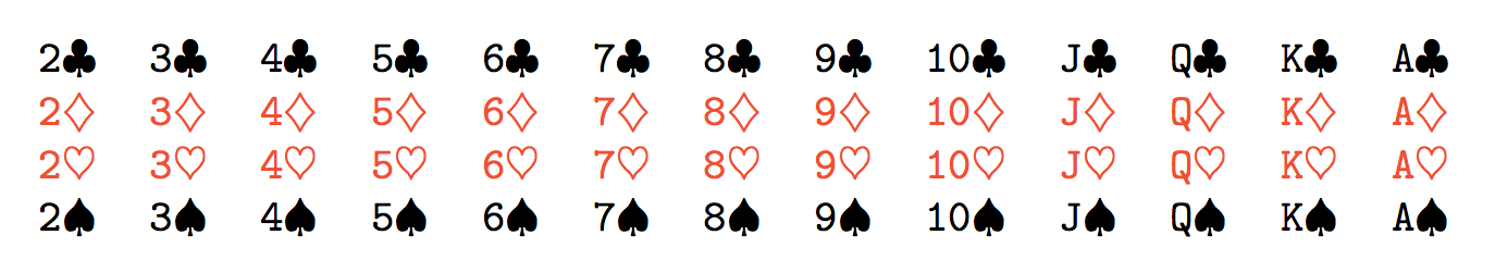
At any rate, it's long standing tradition to use coin flips, dice rolls and cards to illustrate the basic principles of probability so it does help to have a basic familiarity with these things. A deck of cards, for example, consists of 52 playing cards of 13 ranks divided into 4 suits
- 13 ranks: A,2,3,4,5,6,7,8,9,10,J,K,Q
- 4 suits: hearts, diamonds, clubs, spades
When we speak of a "well shuffled deck" we mean that, when we draw one card, each card is equally likely to be drawn. Similarly, when we speak of a fair coin or a fair die, we mean each outcome produced (heads/tails or 1-6) is equally likely to occur.
That brings us our first formula for computing probabilities!
Equal likelihoods
When when the sample space is a finite set and all the individual outcomes are all equally likely, then the probability of an even $A$ can be computed by
$$P(A) = \frac{\# \text{ of possibilities in } A}{\text{total } \# \text{ of possibilities}}.$$Examples: Suppose we draw a card from a well shuffled standard deck of 52 playing cards.
- What's the probability that we draw the four of hearts?
- What's the probability that we draw a four?
- What's the probability that we draw a club?
- What's the probability that we draw a red king?
Mutually exclusive events
The events $A$ and $B$ are called mutually exclusive if only one of them can occur. Another term for this same concept is disjoint. If we know the probability that $A$ occurs and we know the probability that $B$ occurs, then we can compute the probability that $A$ or $B$ occurs by simply adding the probabilities. Symbolically,
$$P(A \text{ or } B) = P(A) + P(B).$$I emphasize, this formula is only valid under the assumption of disjointness.
Examples: We again draw a card from a well shuffled standard deck of 52 playing cards.
- What is the probability that we get an odd numbered playing card?
- What is the probability that we get a face card?
- What is the probability that we get an odd numbered playing card or get a face card?
A more general addition rule
If two events are not mutually exclusive, we have to account for the possibility that both occur. Symbolically:
$$P(A \text{ or } B) = P(A) + P(B) - P(A \text{ and } B).$$Examples: Yet again, we draw a card from a well shuffled standard deck of 52 playing cards.
- What is the probability that we get a face card or we get a red card?
- What is the probability that we get an odd numbered playing or we get a club?
Now, things are getting a little tougher so let's include the computation for that second one right here. Let's define our symbols and say
\begin{align*} A &= \text{we draw an odd numbered card} \\ B &= \text{we draw a club}. \end{align*}In a standard deck, there are four odd numbers we can draw: 3, 5, 7, and 9; and four of each of those for a total of 16 odd numbered cards. Thus, $$P(A) = \frac{16}{52} = \frac{4}{13}.$$ There are also 13 clubs so that $$P(B) = \frac{13}{52} = \frac{1}{4}.$$
Now, there are four odd numbered cards that are clubs - the 3 of clubs, the 5 of clubs, the 7 of clubs, and the 9 of clubs. Thus, the probability of drawing an odd numbered card that is also a club is $$P(A \text{ and } B) = \frac{4}{52} = \frac{1}{13}.$$ Putting this all together, we get $$P(A \text{ or } B) = \frac{4}{13} + \frac{1}{4} - \frac{1}{13} = \frac{25}{52}.$$
Independent events
When two events are independent, we can compute the probability that both occur by multiplying their probabilities. Symbolically, $$P(A \text{ and } B) = P(A)P(B).$$
Examples: Suppose I flip a fair coin twice.
- What's the probability that I get 2 heads?
- What's the probability that I get a head and a tail?
- Now suppose I flip the coin 4 times. What's the probability that I get 4 heads?
Conditional probability
When two events $A$ and $B$ are not independent, we can use a generalized form of the multiplication rule to compute the probability that both occur, namely $$P(A \text{ and } B) = P(A)P(B|A).$$ That last term, $P(B|A)$, denotes the conditional probability that $B$ occurs under the assumption that $A$ occurs.
Example: We draw two cards from a well-shuffled deck. What is the probability that both are hearts?
Solution: The probability of that the first is a heart is $13/52=1/4$. The probability that the second card is a heart is different because we now have a deck with 51 cards and 12 hearts. Thus, the probability of getting a second heart is $12/51 = 4/17$. Thus, the answer to the question is $$\frac{1}{4}\times\frac{4}{17} = \frac{1}{17}.$$ To write this symbolically, we might let
- $A$ denote the event that the first draw is a heart and
- $B$ denote the event that the second draw is a heart.
Then, we express the above as $$P(A \text{ and } B) = P(A)P(B\,|\,A) = \frac{1}{4}\times\frac{4}{17} = \frac{1}{17}.$$
Turning the computation around
Often, it is the computation of conditional probability itself that we are interested in. Thus, we might rewrite our general multiplication rule in the form $$P(B\,|\,A) = \frac{P(A \text{ and } B)}{P(A)}.$$
Example: What is the probability that a card is a heart, given that it's red?
Data
Often, we'd like to compute probabilities from data. For example, here's a contingency table based on our CDC data relating smoking and exercise:
| exer/smoke | 0 | 1 | All |
|---|---|---|---|
| 0 | 0.12715 | 0.12715 | 0.2543 |
| 1 | 0.40080 | 0.34490 | 0.7457 |
| All | 0.52795 | 0.47205 | 1.0000 |
From here, it's pretty easy to read off basic probabilities or compute conditional probabilities. For example, the probability that a someone from this sample exercises is 0.7457. The probability that someone from this sample exercises and smokes is 0.34490.
Conditional probabilities can be computed using the formula $$ P(A|B) = \frac{P(A \cap B)}{P(B)}. $$ For example, the probability that someone smokes, given that they exercise is $$ \frac{0.3449}{0.7457} = 0.462518. $$