Visualizing and describing numerical data
So far, we've met a little bit of data and talked about some techniques to get data. Today, we're going to focus on numerical data and how to visualize and describe it.
This is mostly section 1.6 of our textbook - now, volume 3.
CDC Data
Let's start with a big data set. The Center for Disease Control publishes lots of data obtained through a number of studies. We're going to play with one particular data set obtained from a study called the Behavioral Risk Factor Surveillance System. This is an ongoing process where over 400,000 US adults are interviewed every year. The resulting data file has over 2000 variables ranging from simple descriptors like age and weight, through basic behaviors like activity level and whether the subject smokes to what kind of medical care the subject receives. I've got a subset of this data on my website listing just 8 variables for a random sample of 20000 individuals. Let's start by loading that data set:
import pandas as pd
df = pd.read_csv('https://www.marksmath.org/data/cdc.csv')
print(len(df.height))
df.head()
Most of the variables (ie., the column names) are self-explanatory. My favorite is smoke100, which is a boolean flag indicating whether or not the individual has smoked 100 cigarettes or more throughout their life. You should probably be able to classify the rest as numerical or categorical.
Describing one dimensional, numerical data
Pandas provides a simple way to describe a list of numerical data. Here's a description of the heights in the CDC data, for example:
h = df['height']
h.describe()
Visualizing one dimensional, numerical data
The min, max and percentiles above can be visualized using a box plot.
%matplotlib inline
df.boxplot('height', vert=False, grid=False);

Sometimes, we might want to ignore the outliers.
df.boxplot('height', vert=False, grid=False, showfliers=False);

A more complete picture of the data is provided by a histogram.
h.hist(bins = 20, grid=False, edgecolor='black');

The mean is a measure of location - it tells us where the data is centered.
m = h.mean()
m
Let's see how this fits in with the histogram.
import matplotlib.pyplot as plt
h.hist(bins = 20, grid=False, edgecolor='black');
plt.plot([m,m],[0,5100], 'y--');

The standard deviation tells us how widely spread the data is:
h.std()
To see the effect of standard deviation you really need to compare two or more histograms.

These height histograms displays a class bell shape; they are normally distributed. You can take a look a family of these with this interactive.
It's worth mentioning that there are other types of shapes that can arise.

Scatter plots for 2D data
Finally, we sometimes need to visualize the relationship between variables. The ideal way to do that is with a scatter plot. For example, here's the relationship between height and weight in the CDC data.
df.plot('height', 'weight', 'scatter',
    c=[(0.1,0.1,0.8,0.2)]
);

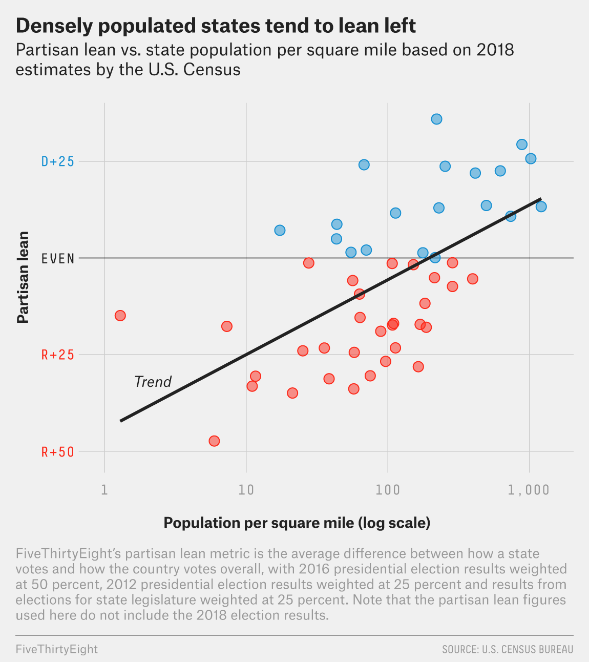
As another example, here's a comparison between population density and partison lean from FiveThirtyEight:
Definitions
Let's take a look at the quantitative definitions of the computational concepts that we've been throwing around above.
The mean and median
Suppose we have a list of numerical data; we'll denote it by $$x_1, x_2, x_3, \ldots, x_n.$$ For example, our list might be $$2, 8, 2, 4, 7.$$ The mean of the list is $$\bar{x} = \frac{x_1 + x_2 + x_3 + \cdots + x_n}{n}.$$ For our concrete example, this is $$\frac{2+8+2+4+7}{5} = \frac{23}{5} = 4.6.$$ The median is the middle value when the list is sorted. For our example, the sorted list is $$2, 2, 4, 7, 8$$ so the median is $4$. If the sorted list has an even number of observations, then the median is the mean of the middle term. For example, the median of $$1,1,3,4,8,8,8,10$$ is the average of $4$ and $8$ which is $6$.
Percentiles (also called quantiles)
- The median is a special case of a percentile - 50% of the population lies below the median and 50% lies above.
- Similarly, 25% of the population lies below the first quartile and 75% lies above.
- Also, 75% of the population lies below the third quartile and 25% lies above.
- The second quartile is just another name for the median.
- The inter-quartile range is the difference between the third and first quartile.
- One reasonable definition of an outlier is a data point that lies more than 3 inter-quartile ranges from the median.
Example
Suppose our data is $$1,2,4,5,5,6,7,9,10.$$ The $25^{\text{th}}$ percentile might be 4, the $75^{\text{th}}$ percentile could be 7 and the inter-quartile range would be 3. There are differing conventions on how you interpolate but these differences diminish with sample size.
Variance and standard deviation
- Percentiles form a measure of the spread of a population or sample related to the median of that population or sample.
- The standard deviation forms a measure of the spread of a population or sample related to the mean of the population or sample.
Definitions
- Roughly, the standard deviation measures how far the individuals deviate from the mean on average.
- The variance is defined to be the square of the standard deviation. Thus, if the standard deviation is $s$, then the variance is $s^2$.
- If we have a sample of $n$ observations $$x_1,x_2,x_3, \ldots, x_n,$$ then the variance is defined by $$s^2 = \frac{(x_1 - \bar{x})^2 + (x_2-\bar{x})^2 +\cdots+(x_n-\bar{x})^2}{n-1}.$$
- If $s^2$ is the variance, then $s$ is the standard deviation.
Sample variance vs population variance
- You might see the definition $$s^2 = \frac{(x_1 - \bar{x})^2 + (x_2-\bar{x})^2 +\cdots+(x_n-\bar{x})^2}{n}.$$
- The difference in the definition is the $n$ in the denominator, rather than $n-1$.
- The difference arises because
- The definition with the $n$ in the denominator is applied to populations and
- The defnition with the $n-1$ in the denominator is applied to samples.
- To make things clear, we will sometimes refer to sample variance vs population variance. More often than not, we will be computing sample variance and the corresponding standard deviation.
Example
Suppose our sample is $$1,2,3,4.$$ Then, the mean is $2.5$ and the variance is $$s^2=\frac{(-3/2)^2 + (-1/2)^2 + (1/2)^2 + (3/2)^2}{3} = \frac{5}{3}.$$ The standard deviation is $$s = \sqrt{5/3} \approx 1.290994.$$