Numerical integration
and the normal distribution
Fri, Feb 27, 2026
Taking stock
Since we just had our first lab (and have already had a couple of “exams”), let’s take a moment to make sure we understand
- the course objective,
- the resulting depth and pace, and
- the resulting approach to exams and labs.
Look ahead
If we take a look at our course calendar, we might notice that our next ML application is logistic regression. The objective of logistic regression is to predict probabilties, as opposed to linear regression where we predicted expected values. Clearly, these should be related and, often, knowledge of expected values can be translated to probabilities.
Consider our Massey ratings, for example, which predict score differences of games. If we think UNCA is going to beat Charleston Southern by 20 tomorrow afternoon, then I guess feel pretty confident in their chances. If we think they’ll win by 1, then we should hedge our bet.
This is exactly what we do in Kaggle’s March Madness competition!
Before we get into all this, though, I guess we need to study some probability theory.
Kaggle-Massey data
Let’s begin by taking a look at some data. This is actual game data (provided by Kaggle) for 3893 NCAA Men’s basketball games that have been played this season. It is current up through Feb 4, 2026.
Residuals
Recall that the idea behind Massey rating is to predict score differences. That is
RatingDiff = Team1MasseyRating - Team2MasseyRating
should project the score.ActualDiff = Team1Score - Team2Score
is the actual score score difference- The difference
ActualDiff - RatingDiffis called the residual.
I guess the sum of the squares of the residuals would be our total squared error.
Histogram
Here’s a histogram of the residuals:
Looks semi-interesting. Almost intriguing!
I wonder if there’s some way to “model” it??
The normal model
Here’s the same histogram, together with its normal model:
We need to understand that curve, which is the normal density function for the data.
Normalization
One very important feature of the histogram is that the areas of the rectangles are scaled so that their total area is \(1\). As a result, we can estimate the proportion of residual values within a certain interval by adding the areas of the rectangles over that interval.
Put another way, if we choose a residual value at random, we can estimate the probability that it lies within a certain interval by finding the areas of the corresponding rectangles.
Similarly, the total area under the curve is \(1\). Furthermore, the curve is “fit” to the data so that the area under the curve and the corresponding area of the rectangles are very close. Thus, we could also compute probabilities using definite integrals.
The normal PDF
The normal Probability Density Function (or PDF) with mean \(\mu\) and standard deviation \(\sigma\) is defined by \[ f_{\mu,\sigma}(x) = \frac{1}{\sqrt{2\pi}\sigma} e^{-(x-\mu)^2/(2\sigma^2)}. \] If we set \(\mu=0\) and \(\sigma=1\), we get the standard normal: \[ f_{0,1}(x) = \frac{1}{\sqrt{2\pi}} e^{-x^2/2}. \]
The family album
Play with the sliders to see that
- \(\mu\) specifies where the mass is concentrated
- \(\sigma\) specifies how concentrated it is.
So…???
Again, we would like to be able to make probabilistic assessments. Here’s an example of the kind of thing we could tackle:
Example
Suppose my computed Massey rating for UNCA is -4.515 and for Ga Southern it’s -9.452. What’s the probability that UNCA wins?
Note that \[ -4.515 - (-9.452) = 4.937 \text{ (or practially }5\text{)} \]
Solution
We have a histogram plotting the data \[ \text{residual } = \text{ actual } - \text{ predicted}. \]
Let’s abbreviate that to \(r=a-p\). These numbers are all known in our data but, now, we’re trying to use them to make a prediction about a game that hasn’t happened yet. That is, we want to know what the actual \(a\) will be. So let’s solve for it: \[ a = p+r. \]
Solution (step 2)
When applying the equation \[ a=p+r, \] \(p\) is known. It’s our prediction arising from the difference in the Massey ratings. The randomness in \(a\) arises from \(r\) and our histogram tells us how \(r\) is distributed.
Now, team 1 wins exactly when \(a=p+r>0\) or \(r>-p\). In our particular case, we need \[ r>-5. \]
Solution (final step 3)
It appears that our question of whether UNCA will defeat Ga Southern boils down to whether a randomly chosen residual \(r\) is larger than \(-5\). We could determine that by simply adding up the areas of the rectangles that lie to the right of \(r=-5\) in the histogram.
More generally, once we have the correct normal distribution function \(f\), we should be able to compute our desired probability as \[ \int_{-5}^{\infty} f(x) \, dx. \]
Challenges and solutions
The challenge
There’s one big, big challenge to this approach: Integration is hard
A solution
In spite of this, we can almost always estimate integrals numerically.
Integration in Python
It’s worth seeing how numerical integration works in a common programming language like Python.
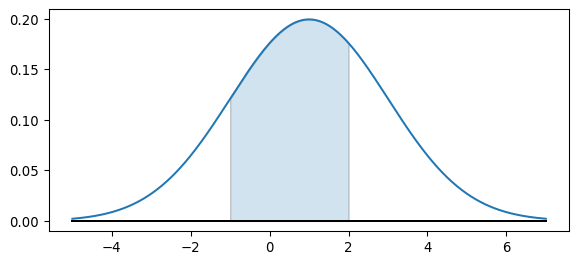
Illustration
Here’s the corresponding picture.
Interesting computations
The total area under the standard normal is \(1\).
\(68\%\) of the population lies within one standard deviation of the mean.