MML Discourse archived in May, 2026

Your personal PCA

mark

(20 pts)

In this problem, you're going to perform PCA on a small data set in 2D.

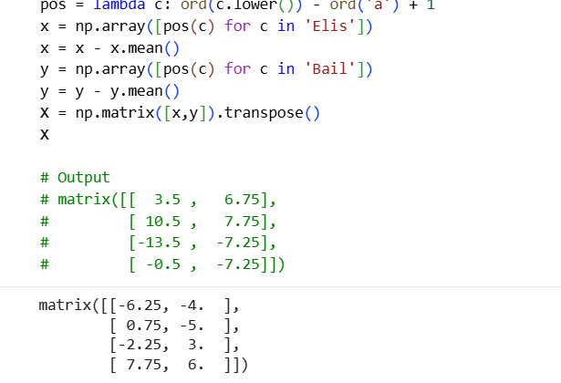
First, generate your data by taking by taking the x coordinates to be the positions in the alphabet of the first four letters in your first name and the y coordinates to be the positions in the alphabet of the first four letters in your last name. These should be the columns of your data matrix.

Then, be sure to center your data. You can use Code like the following to accomplish this:

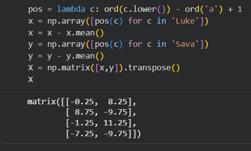
pos = lambda c: ord(c.lower()) - ord('a') + 1
x = np.array([pos(c) for c in 'Mark'])
x = x - x.mean()
y = np.array([pos(c) for c in 'McCl'])
y = y - y.mean()
X = np.matrix([x,y]).transpose()
X

# Output:
# matrix([[ 2.25,  5.25],
#   [-9.75, -4.75],
#   [ 7.25, -4.75],
#   [ 0.25,  4.25]
# ])

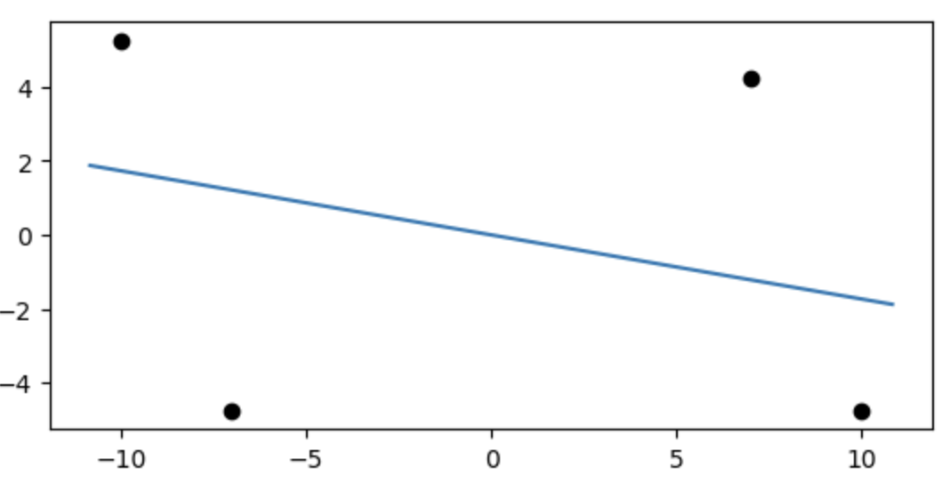
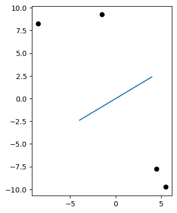
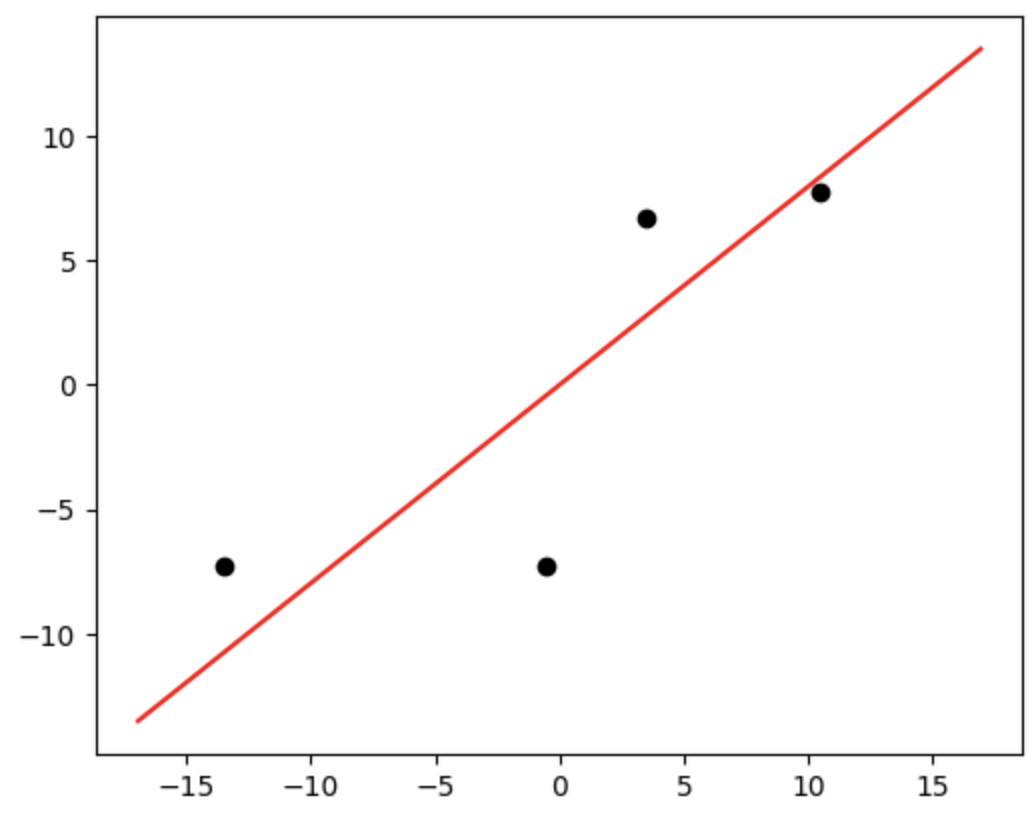
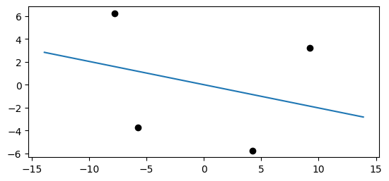
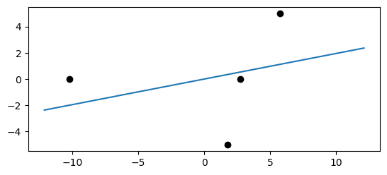
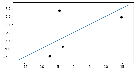
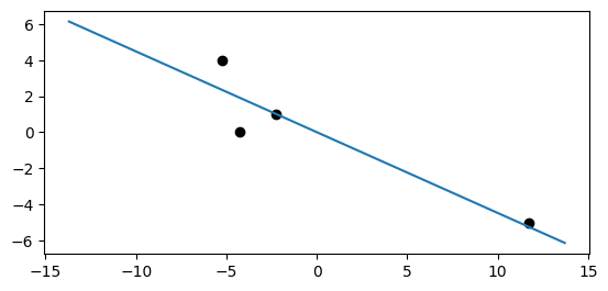
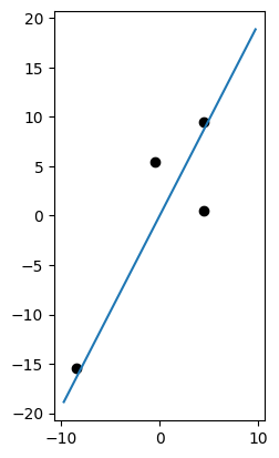
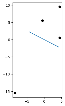
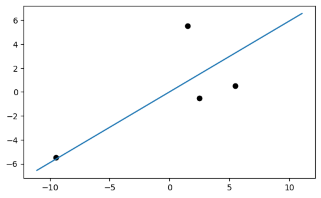
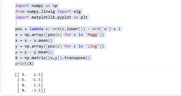
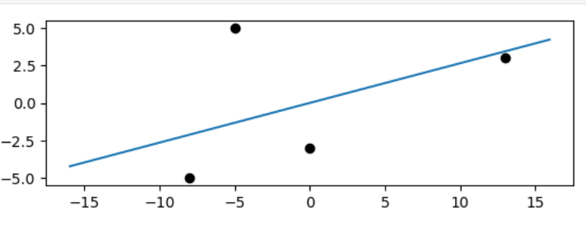
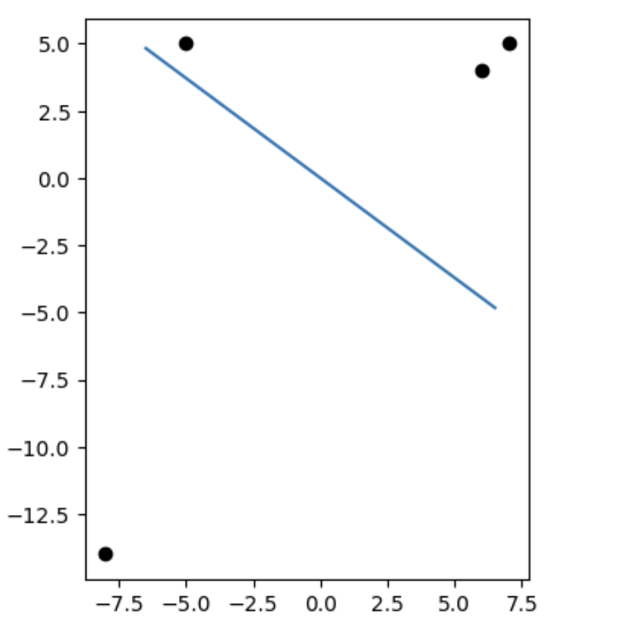
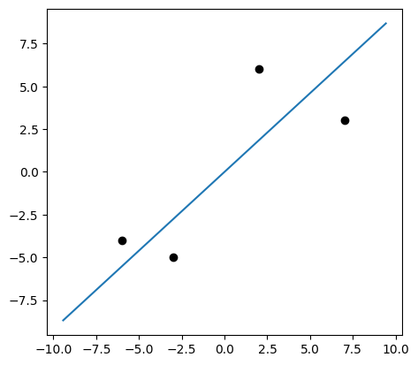
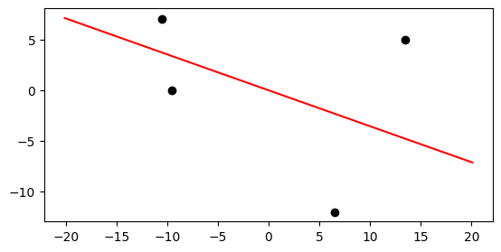
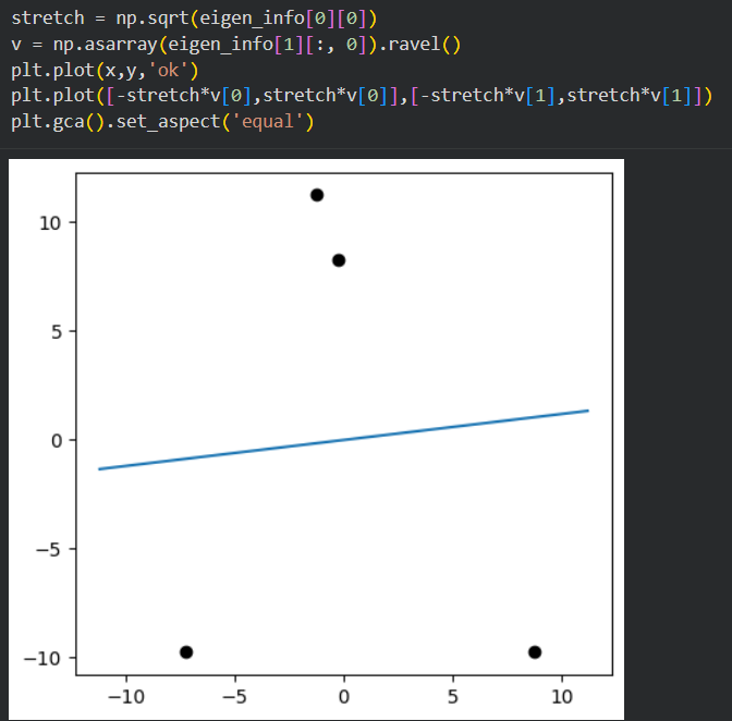
Once you've set up your matrix, you can modify the code in this column of slides to perform to PCA. When responding to this post, be sure to show all the code that

defines your matrix,
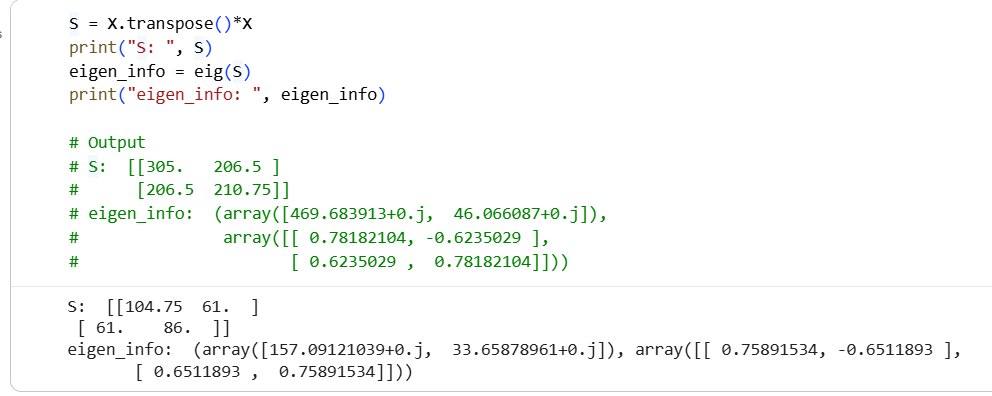
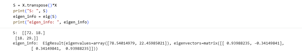
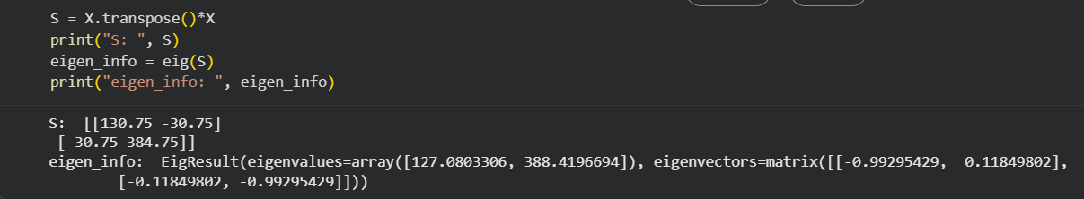
computes the principal components, and
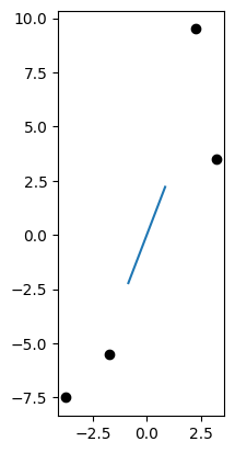
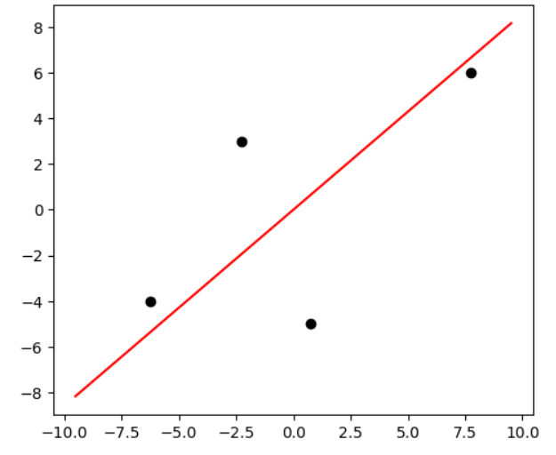
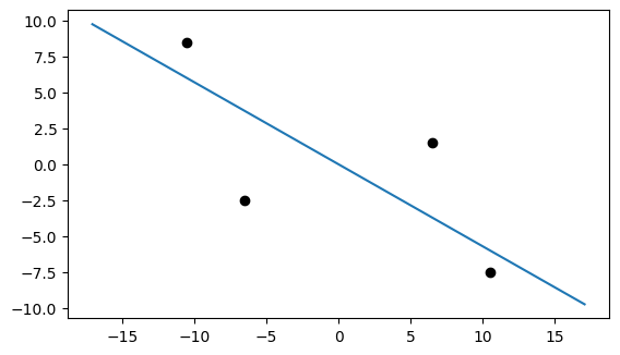
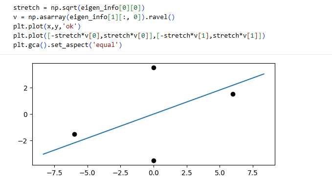
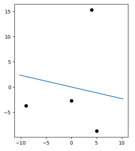
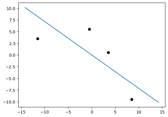
plots the data together with a line showing the direction of the first principal component.

Finally, indicate the variance in the directions of those first two principal components.

👍 1

audrey

The first four letters of my first and last name are

Audr McCl

Using the code provided (and importing the proper libraries) I get the following matrix:

import numpy as np
from numpy.linalg import eig
import matplotlib.pyplot as plt

pos = lambda c: ord(c.lower()) - ord('a') + 1
x = np.array([pos(c) for c in 'Audr'])
x = x - x.mean()
y = np.array([pos(c) for c in 'McCl'])
y = y - y.mean()
X = np.matrix([x,y]).transpose()
X

# Output:
# matrix([
#   [-10.  ,   5.25],
#   [ 10.  ,  -4.75],
#   [ -7.  ,  -4.75],
#   [  7.  ,   4.25]
# ])

Now, to compute the eigenvalue info, I use the code provided in the column of slides that Mark referenced:

S = X.transpose()*X
print("S: ", S)
eigen_info = eig(S)
print("eigen_info: ", eigen_info)

# Printout
# S:  [
#  [298.   -37.  ]
#  [-37.    90.75]
# ]
# eigen_info: EigResult(
#   eigenvalues=array([304.4074526,  84.3425474]),
#   eigenvectors=matrix([
#     [ 0.98533436,  0.17063468],
#     [-0.17063468,  0.98533436]
#   ])
# )

From that information, I can see that the first principal component is determined by the vector

\mathbf{v} = \begin{bmatrix}0.98533436 & -0.17063468\end{bmatrix}^{\mathsf{T}}

and that the variance of the data in that direction is about \frac{1}{4} \times 304.4074526.

Finally, here a plot of the data together with the line spanned by that first principal component:

stretch = np.sqrt(eigen_info[0][0])
v = np.asarray(eigen_info[1][:, 0]).ravel()
plt.plot(x,y,'ok')
plt.plot([-stretch*v[0],stretch*v[0]],[-stretch*v[1],stretch*v[1]])
plt.gca().set_aspect('equal')

Here's a link to the notebook:

User 002

The first four letters of my first and last name are Noah Cast.
I used the code provided:

import numpy as np
from numpy.linalg import eig
import matplotlib.pyplot as plt

pos = lambda c: ord(c.lower()) - ord('a') + 1

x = np.array([pos(c) for c in 'Noah'])
x = x - x.mean()
y = np.array([pos(c) for c in 'Cast'])
y = y - y.mean()

X = np.matrix([x,y]).transpose()
X

S = X.transpose()*X
print("S: ", S)

eigen_info = eig(S)
print("eigen_info: ", eigen_info)

Here's the output:

S:  [[ 125.   -172.5 ]
 [-172.5   308.75]]
eigen_info:  EigResult(eigenvalues=array([ 21.43379241, 412.31620759]), eigenvectors=matrix([[-0.85734772,  0.51473769],
        [-0.51473769, -0.85734772]]))

From that information, I can see that the first principal component is determined by the vector

\mathbf{v} = \begin{bmatrix} -0.85734772, -0.51473769 \end{bmatrix}^{T}

and that the variance of the data is about (1/4) \times 21.43379241.
Finally, here is a plot of the data together with the line spanned by that first principal component:

stretch = np.sqrt(eigen_info[0][0])
v = np.asarray(eigen_info[1][:, 0]).ravel()
plt.plot(x,y,'ok')
plt.plot([-stretch*v[0],stretch*v[0]],[-stretch*v[1],stretch*v[1]])
plt.gca().set_aspect('equal')

Colab notebook: Google Colab

❤️ 2

User 003

The first 4 letters of my first and last name are:

ryan stee

My matrix of centered data is defined as follows.

pos = lambda c: ord(c.lower()) - ord('a') + 1
x = np.array([pos(c) for c in 'Ryan'])
x = x - x.mean()
y = np.array([pos(c) for c in 'Stee'])
y = y - y.mean()
X = np.matrix([x,y]).transpose()
X

# Output
# matrix([[  3.5 ,   6.75],
#         [ 10.5 ,   7.75],
#         [-13.5 ,  -7.25],
#         [ -0.5 ,  -7.25]])

Eigenvalues and eigenvectors are found from the covariance matrix, S, is defined as follows.

S = X.transpose()*X
print("S: ", S)
eigen_info = eig(S)
print("eigen_info: ", eigen_info)

# Output
# S:  [[305.   206.5 ]
#      [206.5  210.75]]
# eigen_info:  (array([469.683913+0.j,  46.066087+0.j]), 
#               array([[ 0.78182104, -0.6235029 ],
#                      [ 0.6235029 ,  0.78182104]]))

The eigenvector associated with the largest eigenvalue (i.e., maximum variance) is

\mathbf{v}=\begin{bmatrix}0.78182104 & 0.6235029\end{bmatrix}^{\mathsf{T}}

with a variance in that direction of \frac{1}{4} \times 469.683913.

Here's the plot showing the data and the first principal component.

#PC1
v1 = np.asarray(eigen_info[1][:, 0]).ravel()
s1 = np.sqrt(eigen_info[0][0])

#PC2
#v2 = np.asarray(eigen_info[1][:, 1]).ravel()
#s2 = np.sqrt(eigen_info[0][1])

plt.plot(x,y,'ok')
plt.plot([-s1*v1[0],s1*v1[0]],[-s1*v1[1],s1*v1[1]],'r')
#plt.plot([-s2*v2[0],s2*v2[0]],[-s2*v2[1],s2*v2[1]],'b')
plt.gca().set_aspect('equal')

And here's the notebook:
https://colab.research.google.com/drive/1dK2zFC_pIDHWcoW_VDTpcKIDB0-T3vlu?usp=sharing

❤️ 1

User 004

The first four letters of my first and last name are

Marc Cole

Using the code provided I get the following matrix

pos = lambda c: ord(c.lower()) - ord('a') + 1
x = np.array([pos(c) for c in 'marc'])
x = x - x.mean()
y = np.array([pos(c) for c in 'cole'])
y = y - y.mean()
X = np.matrix([x,y]).transpose()
X
#Output:
#matrix([[ 4.25, -5.75],
#        [-7.75,  6.25],
#        [ 9.25,  3.25],
#        [-5.75, -3.75]])

Here's the computed eigenvalues of this info

S = X.transpose()*X
print("S: ", S)
eigen_info = eig(S)
print("eigen_info: ", eigen_info)

#Printout:
#S:  [[196.75 -21.25]
#     [-21.25  96.75]]
#eigen_info:  EigResult(eigenvalues=array([201.07828453,  92.42171547]), eigenvectors=matrix([
#                     [ 0.97988033,  0.19958592],
#                     [-0.19958592,  0.97988033]
#]))

From this information, the first principal component is determined by the vector:

\mathbf{v} = \begin{bmatrix}0.97988033, -0.19958592\end{bmatrix}^T

and that the variance of the data is about \frac{1}{4} \times 201.07828453.

Here is the data plotted by the line spanned by the first principal component:

stretch = np.sqrt(eigen_info[0][0])
v = np.asarray(eigen_info[1][:, 0]).ravel()
plt.plot(x,y,'ok')
plt.plot([-stretch*v[0],stretch*v[0]],[-stretch*v[1],stretch*v[1]])
plt.gca().set_aspect('equal')

Heres the notebook:
Another copy of FundamentalPCA.ipynb - Colab

❤️ 1

User 005

The first four letters of my first and last name are

John Clar

Using the code provided (and importing the proper libraries) I get the following matrix:

import numpy as np
from numpy.linalg import eig
import matplotlib.pyplot as plt

pos = lambda c: ord(c.lower()) - ord('a') + 1
x = np.array([pos(c) for c in 'John'])
x = x - x.mean()
y = np.array([pos(c) for c in 'Clar'])
y = y - y.mean()
X = np.matrix([x,y]).transpose()
X

# Output:
# matrix([[-1.75,  -5.5 ],
#   [ 3.25,  3.5 ],
#   [-3.75, -7.5 ],
#   [ 2.25,  9.5 ]
# ])

Now, to compute the eigenvalue info, I use the code provided in the column of slides that Dr. McClure referenced:

S = X.transpose()*X
print("S: ", S)
eigen_info = eig(S)
print("eigen_info: ", eigen_info)

# Printout
# S:  [
#  [ 32.75  70.5 ]
#  [ 70.5  189.  ]
# ]
# eigen_info: EigResult(
#   eigenvalues=array([  5.64303896, 216.10696104]),
#   eigenvectors=matrix([
#     [-0.93338297, -0.35888193],
#     [ 0.35888193, -0.93338297]
#   ])
# )

From that information, I can see that the first principal component is determined by the vector

v=[-0.93338297, 0.35888193]^T

and that the variance of the data in that direction is about 1/4 * 5.64303896.

Finally, here is a plot of the data together with the line spanned by that first principal component:

stretch = np.sqrt(eigen_info[0][0])
v = np.asarray(eigen_info[1][:, 1]).ravel()
plt.plot(x,y,'ok')
plt.plot([-stretch*v[0],stretch*v[0]],[-stretch*v[1],stretch*v[1]])
plt.gca().set_aspect('equal')

Here's a link to the notebook:
Google Colab

❤️ 1

mark

Does that look like the direction of greatest variance?

Looks much better now!

User 006

The first four letters of my first and last name are
Elis Bail

I used the code provided and got the following matrix:

My next step was using the code provided in the slides by Dr. McClure

I can see the PCA is determined by the vector

V = [0.75891534, 0.6511893 ]

❤️ 1

User 007

The first four letters of my first and last name are Quet Kupp

import numpy as np
from numpy.linalg import eig
import matplotlib.pyplot as plt

pos = lambda c: ord(c.lower()) - ord('a') + 1
x = np.array([pos(c) for c in 'Quer'])
x = x - x.mean()
y = np.array([pos(c) for c in 'Kupp'])
y = y - y.mean()
X = np.matrix([x,y]).transpose()
X

T = X.transpose() * X
print("T: ", T)
print()
eigen_info = eig(T)
print("eigen_info: ", eigen_info)

Output:

T:  [[148.75  20.  ]
 [ 20.    50.  ]]

eigen_info:  EigResult(eigenvalues=array([152.64685584,  46.10314416]), eigenvectors=matrix([[ 0.98154206, -0.1912464 ],
        [ 0.1912464 ,  0.98154206]]))

v= [0.1912464 , 0.98154206]

and the Variance of the data is about 1/4 * 152.64685584.

And Now finlay the graph with the plot of the data together

stretch = np.sqrt(eigen_info[0][0])
v = np.asarray(eigen_info[1][:, 0]).ravel()
plt.plot(x,y,'ok')
plt.plot([-stretch*v[0],stretch*v[0]],[-stretch*v[1],stretch*v[1]])
plt.gca().set_aspect('equal')

❤️ 1

User 008

My name's first 4: Edwa Doma

Define the matrix:

import numpy as np
from numpy.linalg import eig
import matplotlib.pyplot as plt

pos = lambda c: ord(c.lower()) - ord('a') + 1
x = np.array([pos(c) for c in 'Edwa'])
x = x - x.mean()
y = np.array([pos(c) for c in 'Doma'])
y = y - y.mean()
X = np.matrix([x,y]).transpose()
X

# Output:
# matrix([[-3.25, -4.25],
#        [-4.25,  6.75],
#        [14.75,  4.75],
#        [-7.25, -7.25]])

Compute Principal Components:

S = X.transpose()*X
print("S: ", S)
eigen_info = eig(S)
print("eigen_info: ", eigen_info)

"""
Output:
S:  [[298.75 107.75]
 [107.75 138.75]]
eigen_info:  EigResult(eigenvalues=array([352.95157413,  84.54842587]), eigenvectors=matrix([[ 0.89334153, -0.44937835],
        [ 0.44937835,  0.89334153]]))
"""

Plotted data with line showing direction of first principal component:

stretch = np.sqrt(eigen_info[0][0])
v = np.asarray(eigen_info[1][:, 0]).ravel()
plt.plot(x,y,'ok')
plt.plot([-stretch*v[0],stretch*v[0]],[-stretch*v[1],stretch*v[1]])
plt.gca().set_aspect('equal')

❤️ 1

User 009

Define Matrix:

import numpy as np
from numpy.linalg import eig
import matplotlib.pyplot as plt

pos = lambda c: ord(c.lower()) - ord('a') + 1
x = np.array([pos(c) for c in 'Brad'])
x = x - x.mean()
y = np.array([pos(c) for c in 'Jenk'])
y = y - y.mean()
X = np.matrix([x,y]).transpose()
X

# Output:
# matrix([[-4.25, 0],
#        [11.75, -5],
#        [-5.25,  4],
#        [-2.25, 1]])

Compute Principal Components

`S = X.transpose()*X
print("S: ", S)
eigen_info = eig(S)
print("eigen_info: ", eigen_info)

"""
Output:
S:  [[188.75 -82]
 [-82 42]]
eigen_info:  EigResult(eigenvalues=array([225.41086063,   5.33913937]), eigenvectors=matrix([[ 0.91291513,  0.40814944],
        [-0.40814944,  0.91291513]]))
"""`
Plotted data with line showing direction of first principal component:

❤️ 1

User 010

First letters of my name: Merr Vazq
Matrix:

import numpy as np
from numpy.linalg import eig
import matplotlib.pyplot as plt

pos = lambda c: ord(c.lower()) - ord('a') + 1
x = np.array([pos(c) for c in 'Merr'])
x = x - x.mean()
y = np.array([pos(c) for c in 'Vazq'])
y = y - y.mean()
X = np.matrix([x,y]).transpose()
X
matrix([[ -0.5,   5.5],
        [ -8.5, -15.5],
        [  4.5,   9.5],
        [  4.5,   0.5]])

PCA:

S = X.transpose()*X
print("S: ", S)
eigen_info = eig(S)
print("eigen_info: ", eigen_info)

S:  [[113. 174.]
 [174. 361.]]
eigen_info:  EigResult(eigenvalues=array([ 23.3367135, 450.6632865]), eigenvectors=matrix([[-0.88891855, -0.45806528],
        [ 0.45806528, -0.88891855]]))

The first principal component is determined by the vector:

v = [-0.4581,-0.8889]

Plot:

stretch = np.sqrt(eigen_info[0][-1])
v = np.asarray(eigen_info[1][:, 1]).ravel()
plt.plot(x,y,'ok')
plt.plot([-stretch*v[0],stretch*v[0]],[-stretch*v[1],stretch*v[1]])
plt.gca().set_aspect('equal')

Colab Notebook
Google Colab

❤️ 1

mark

@User 011 This doesn't look like the first principal component to me:

image253×413 4.78 KB

It looks like the second principal component.

Note that the mathematical eigenvectors are the columns of the matrix presented in the Python eigen_info.eigenvecotrs object. The order is determiend by the eigenvalues array. You want the larger of the two, which looks like the second eigenvalue, rather than the first.

The upshot is, that you want

v = np.asarray(eigen_info[1][:, 1]).ravel()

rather than

v = np.asarray(eigen_info[1][:, 0]).ravel()

User 012

The first four letters of my first and last name are

Corn Chin

Using the code provided defines the following matrix:

import numpy as np
from numpy.linalg import eig
import matplotlib.pyplot as plt

pos = lambda c: ord(c.lower()) - ord('a') + 1
x = np.array([pos(c) for c in 'Corn'])
x = x - x.mean()
y = np.array([pos(c) for c in 'Chin'])
y = y - y.mean()
X = np.matrix([x,y]).transpose()
X

# Output:
# matrix([[-9.5, -5.5],
#        [ 2.5, -0.5],
#        [ 5.5,  0.5],
#        [ 1.5,  5.5]])

Now, to compute the eigenvalue info from the covariance matrix S:

S = X.transpose()*X
print("S: \n", S)
eigen_info = eig(S)
print("eigen_info: ", eigen_info)

# Output:
# S: 
# [[129.  62.]
# [ 62.  61.]]
# eigen_info:  EigResult(
# eigenvalues=array([165.71067812,  24.28932188]), 
# eigenvectors=matrix([[ 0.86047447, -0.50949357],
#                      [ 0.50949357,  0.86047447]]))

From that information, I can see the first principal component is determined by the vector

v = [0.86047447 \quad 0.50949357]^{\intercal}

and that the variance of the data in that direction is about \frac{1}{4}\times 165.71067812.

Finally, here a plot of the data together with the line spanned by that first principal component:

stretch = np.sqrt(eigen_info[0][0])
v = np.asarray(eigen_info[1][:, 0]).ravel()
plt.plot(x,y,'ok')
plt.plot([-stretch*v[0],stretch*v[0]],[-stretch*v[1],stretch*v[1]])
plt.gca().set_aspect('equal')

Here's a link to the notebook:
https://colab.research.google.com/drive/1BV-tCOnJzWz2lSjrdkmc3Pzj_uQsUSXQ?usp=sharing

❤️ 1

User 013

The first 4 letters of my first and last name are
Aida Tobb

This is the matrix using the code provided:

x = np.array([pos(c) for c in 'Aida'])
x = x - x.mean()
y = np.array([pos(c) for c in 'Tobb'])
y = y - y.mean()
X = np.matrix([x,y]).transpose()
X 

matrix([[-2.75, 10.25],
        [ 5.25,  5.25],
        [ 0.25, -7.75],
        [-2.75, -7.75]])

Now to calculate the eigenvalues and vectors:

print("S: ", S)
eigen_info = eig(S)
print("eigen_info: ", eigen_info)

S:  [[ 42.75  18.75]
 [ 18.75 252.75]]
eigen_info:  EigResult(eigenvalues=array([ 41.0890301, 254.4109699]), eigenvectors=matrix([[-0.99609929, -0.08823952],
        [ 0.08823952, -0.99609929]]))

That tells me that the first principal component is determined by the vector

v =[0.98533436−0.17063468]^T

and that the variance of the data in that direction is about

14×304.4074526

Here is the plotted graph

❤️ 1

User 014

The first four letters of my first and last name are

Anis Golr

Using the code provided, I get the following matrix:

import numpy as np
from numpy.linalg import eig
import matplotlib.pyplot as plt

pos = lambda c: ord(c.lower()) - ord('a') + 1
x = np.array([pos(c) for c in 'Anis'])
x = x - x.mean()
y = np.array([pos(c) for c in 'Golr'])
y = y - y.mean()
X = np.matrix([x,y]).transpose()
X
# matrix([[-9.75, -6.  ],
#        [ 3.25,  2.  ],
#        [-1.75, -1.  ],
#        [ 8.25,  5.  ]])

The computed eigenvalues are:

S = X.transpose()*X
print("S: ", S)
eigen_info = eig(S)
print("eigen_info: ", eigen_info)

# S:  [[176.75 108.  ]
# [108.    66.  ]]
# eigen_info:  EigResult(eigenvalues=array([2.42743821e+02, 6.17935400e-03]), eigenvectors=matrix([[ 0.85330356, -0.52141446],
#        [ 0.52141446,  0.85330356]]))

From this, the first principal component is determined by the vector:

\mathbf{v} = \begin{bmatrix} 0.85330356, \ 0.52141446 \end{bmatrix}^T

and the variance of the data is

\sim \frac{1}{4} \cdot 2.42743821 \times 10^{2}.

Here's the plot showing the data and first principal component:

stretch = np.sqrt(eigen_info[0][0])
v = np.asarray(eigen_info[1][:, 0]).ravel()
plt.plot(x,y,'ok')
plt.plot([-stretch*v[0],stretch*v[0]],[-stretch*v[1],stretch*v[1]])
plt.gca().set_aspect('equal')

❤️ 1

User 015

The first four letters of my first and last name are

Aver Schl

Using the code provided, I get the following matrix:

pos = lambda c: ord(c.lower()) - ord('a') + 1
x = np.array([pos(c) for c in 'Aver'])
x = x - x.mean()
y = np.array([pos(c) for c in 'Schl'])
y = y - y.mean()
X = np.matrix([x,y]).transpose()
X

# Output:
# matrix([[-10.5,   8.5],
        # [ 10.5,  -7.5],
        # [ -6.5,  -2.5],
        # [  6.5,   1.5]])

To compute the eigenvalue info, I use the code provided in the Lecture 19 slides:

S = X.transpose()*X
print("S: ", S)
eigen_info = eig(S)
print("eigen_info: ", eigen_info)

#Output:
# S:  [[ 305. -142.]
#  [-142.  137.]]
# eigen_info:  (array([385.98484779+0.j,  56.01515221+0.j]), array([[ 0.86865922,  0.4954101 ],
#        [-0.4954101 ,  0.86865922]]))

From that information, I can see that the first principal component is determined by the vector

\mathbf{v} = \begin{bmatrix}0.86865922 & 0.4954101 \end{bmatrix}^{\mathsf{T}}

Here a plot of the data together with the line spanned by that first principal component:

stretch = np.sqrt(eigen_info[0][0])
v = np.asarray(eigen_info[1][:, 0]).ravel()
plt.plot(x,y,'ok')
plt.plot([-stretch*v[0],stretch*v[0]],[-stretch*v[1],stretch*v[1]])
plt.gca().set_aspect('equal')

Here is the link to the Colab notebook

❤️ 1

User 016

The first four letters of my first and last name are Magg Ling

Using the code I get

and

From that information, I can see that the first principal component is determined by the vector

𝐯=[0.98533436 −0.17063468]T

and that the variance of the data in that direction is about 1/4 * 64.694
Here is a plot of my data with the PCA line

❤️ 1

User 017

The first four letters of my first and last names are

Davi McKe

Using the code provided (and importing the proper libraries), I get the following matrix:

python

import numpy as np
from numpy.linalg import eig
import matplotlib.pyplot as plt

pos = lambda c: ord(c.lower()) - ord('a') + 1
x = np.array([pos(c) for c in 'Davi'])
x = x - x.mean()
y = np.array([pos(c) for c in 'McKe'])
y = y - y.mean()
X = np.matrix([x,y]).transpose()
X

# Output:
# matrix([[-5.,  5.],
#         [-8., -5.],
#         [13.,  3.],
#         [ 0., -3.]])

Now, to compute the eigenvalue info, I use the code provided in the column of slides:

python

S = X.transpose()*X
print("S: ", S)
eigen_info = eig(S)
print("eigen_info: ", eigen_info)

# Output:
# S:  [[258.  54.]
#      [ 54.  68.]]
# eigen_info: EigResult(
#   eigenvalues=array([272.27488275,  53.72511725]),
#   eigenvectors=matrix([[ 0.96679036, -0.25557072],
#                       [ 0.25557072,  0.96679036]]))

From that information, I can see that the first principal component is determined by the vector v = [0.96679036, 0.25557072]ᵀ

and that the variance of the data in that direction is about (1/4) × 272.27488275. The variance in the direction of the second principal component is about (1/4) × 53.72511725.

Finally, here is a plot of the data together with the line spanned by that first principal component:

python

stretch = np.sqrt(eigen_info[0][0])
v = np.asarray(eigen_info[1][:, 0]).ravel()
plt.plot(x,y,'ok')
plt.plot([-stretch*v[0],stretch*v[0]],[-stretch*v[1],stretch*v[1]])
plt.gca().set_aspect('equal')

❤️ 1

User 001

The first four letter for my name are Seth Satt.

import numpy as np

from numpy.linalg import eig

import matplotlib.pyplot as plt

pos = lambda c: ord(c.lower()) - ord('a') + 1

x = np.array([pos(c) for c in 'Seth'])

x = x - x.mean()

y = np.array([pos(c) for c in 'Satt'])

y = y - y.mean()

X = np.matrix([x,y]).transpose()

X

Output:

matrix([[  6.,   4.],
        [ -8., -14.],
        [  7.,   5.],
        [ -5.,   5.]])

S = X.transpose()*X

print("S: ", S)

eigen_info = eig(S)

print("eigen_info: ", eigen_info)

Output:

S:  [[174. 146.]
 [146. 262.]]
eigen_info:  EigResult(eigenvalues=array([ 65.51393506, 370.48606494]), eigenvectors=matrix([[-0.80266773, -0.59642646],
        [ 0.59642646, -0.80266773]]))

From this I can see the first principal component is
𝐯=[ -0.80266773 0.59642646]𝖳

Link to the notebook:

❤️ 1

User 018

My first four letters are Dani DeLo

I used the code:

import numpy as np
from numpy.linalg import eig
import matplotlib.pyplot as plt

pos = lambda c: ord(c.lower()) - ord('a') + 1
x = np.array([pos(c) for c in 'Dani'])
x = x - x.mean()
y = np.array([pos(c) for c in 'Delo'])
y = y - y.mean()
X = np.matrix([x,y]).transpose()
X

#
#matrix([[-3., -5.],
#        [-6., -4.],
#        [ 7.,  3.],
#        [ 2.,  6.]])
#
#

To get the eigenvalue info I used the code:

S = X.transpose()*X
print("S: ", S)
eigen_info = eig(S)
print("eigen_info: ", eigen_info)

S:  [[98. 72.]
 [72. 86.]]
eigen_info:  EigResult(eigenvalues=array([164.24956747,  19.75043253]), eigenvectors=matrix([[ 0.73588229, -0.67710949],
        [ 0.67710949,  0.73588229]]))

The first principal component is determined by the vector

[0.73588229,0.67710949]^{\!\!T}

and the variance is about

\frac14\cdot164.24956747.

Here is the plot of data with the line spanned by that first principal component:

stretch = np.sqrt(eigen_info[0][0])
v = np.asarray(eigen_info[1][:, 0]).ravel()
plt.plot(x,y,'ok')
plt.plot([-stretch*v[0],stretch*v[0]],[-stretch*v[1],stretch*v[1]])
plt.gca().set_aspect('equal')

https://colab.research.google.com/drive/1eCsJx4U1Ur75Z7Fu5TzcqlkL0pGrzXfU?usp=sharing

❤️ 1

User 019

The first four letters of my first and last name are:

Brya Mart

Using the code providing, I get the following matrix:

import numpy as np
from numpy.linalg import eig
import matplotlib.pyplot as plt

pos = lambda c: ord(c.lower()) - ord('a') + 1

x = np.array([pos(c) for c in 'Brya'])
x = x - x.mean()

y = np.array([pos(c) for c in 'Mart'])
y = y - y.mean()

X = np.matrix([x, y]).transpose()
print(X)

#Output:
#[[ -9.5   0. ]
# [  6.5 -12. ]
# [ 13.5   5. ]
# [-10.5   7. ]]

Now, to the compute the eigenvalue info, I used the code provided in the slides:

S = X.transpose() * X
print("S:", S)

eigen_info = eig(S)
print("eigen_info:", eigen_info)

"""
Output: 

S: [[425. -84.]
 [-84. 218.]]
eigen_info: EigResult(eigenvalues=array([454.79759938, 188.20240062]), eigenvectors=matrix([[ 0.94245904,  0.33432163],
        [-0.33432163,  0.94245904]]))

"""

From that information, I can see that the first principal component is determined by the vector

[0.94245904, -0.33432163]^T

and the variance of the data is about \frac{1}{4} (454.79759938) \approx 113.6994.
Finally, here is a plot of the data together with the line spanned by the first principal component:

v1 = np.asarray(eigen_info[1][:, 0]).ravel()
s1 = np.sqrt(eigen_info[0][0])

plt.plot(x, y, 'ok')
plt.plot([-s1*v1[0], s1*v1[0]], [-s1*v1[1], s1*v1[1]], 'r')
plt.gca().set_aspect('equal')
plt.show()

Link to the notebook:

❤️ 1

User 020

The first four letters of my first and last name are:

Jona Gayf

Using the code provided and proper libraries I get the following matrix:

import numpy as np
from numpy.linalg import eig
import matplotlib.pyplot as plt
pos = lambda c: ord(c.lower()) - ord('a') + 1
x = np.array([pos(c) for c in 'Jona'])
x = x - x.mean()
y = np.array([pos(c) for c in 'Gayf'])
y = y - y.mean()
X = np.matrix([x,y]).transpose()
X

matrix([[ 0. , -2.75],
[ 5. , -8.75],
[ 4. , 15.25],
[-9. , -3.75]])

Using this code from slides referenced:

S = X.transpose()*X
print("S: ", S)
eigen_info = eig(S)
print("eigen_info: ", eigen_info)

We get the following results for eigenvalues and vectors:

S: [[122. 51. ]
[ 51. 330.75]]
eigen_info: EigResult(eigenvalues=array([110.20641292, 342.54358708]), eigenvectors=matrix([[-0.97428915, -0.22530125],
[ 0.22530125, -0.97428915]]))

I can see that the first principal component is given by:

v = [-0.97428915, -0.22530125]^T

and the variance of the data in that direction is:

\frac{1}{4} \cdot 110.20641292

Finally, using this code we plot the data to get a line spanned by the first principal component:

stretch = np.sqrt(eigen_info[0][0])
v = np.asarray(eigen_info[1][:, 0]).ravel()
plt.plot(x,y,'ok')
plt.plot([-stretch*v[0],stretch*v[0]],[-stretch*v[1],stretch*v[1]])
plt.gca().set_aspect('equal')

Here is the link to the colab book:

❤️ 1

User 021

The first four letters of my first and last name are

Paul Knap

Using the code provided (and importing the proper libraries) I get the following matrix:

pos = lambda c: ord(c.lower()) - ord('a') + 1
x = np.array([pos(c) for c in 'Paul'])
x = x - x.mean()
y = np.array([pos(c) for c in 'Knap'])
y = y - y.mean()
X = np.matrix([x,y]).transpose()
X

#Output
#matrix([[  3.5,   0.5],
#        [-11.5,   3.5],
#        [  8.5,  -9.5],
#        [ -0.5,   5.5]])

Now, to compute the eigenvalue info, I use the code provided in the column of slides that Mark referenced:

S = X.transpose()*X
print("S: ", S)
eigen_info = eig(S)
print("eigen_info: ", eigen_info)

# Printout
# S:  [[ 217. -122.]
# [-122.  133.]]
#eigen_info:  EigResult(eigenvalues=array([304.02712893,  45.97287107]), #eigenvectors=matrix([[ 0.81409856,  0.58072673],
#        [-0.58072673,  0.81409856]]))

From that information, I can see that the first principal component is determined by the vector v = [0.81409856, 0.58072673]^T.
and that the variance of the data in that direction is about 1/4 * 304.02712893.

Finally, here a plot of the data together with the line spanned by that first principal component:

stretch = np.sqrt(eigen_info[0][0])
v = np.asarray(eigen_info[1][:, 0]).ravel()
plt.plot(x,y,'ok')
plt.plot([-stretch*v[0],stretch*v[0]],[-stretch*v[1],stretch*v[1]])
plt.gca().set_aspect('equal')