From the three data points given, we have the vectors:
\mathbf{x}=[1,2,3]^\mathsf{T} where the mean (µ_x) = 2, and
\mathbf{y}=[0,2,1]^\mathsf{T} where the mean (µ_y) = 1
To center the data, we subtract the mean from each element, so the centered vectors are:
\mathbf{x}=[-1,0,1]^\mathsf{T}
\mathbf{y}=[-1,1,0]^\mathsf{T}
which we can put into the matrix \mathbf{X}:
\mathbf{X} = \begin{bmatrix}-1 & -1\\ 0 & 1 \\ 1 & 0\end{bmatrix}
Principal components are the eigenvectors (\mathbf{v}) of the covariance matrix \mathbf{X}^\mathsf{T}\mathbf{X}.
First, finding the eigenvalues:
(\mathbf{X}^\mathsf{T}\mathbf{X}-\lambda I)\mathbf{v}=\mathbf{0}
(\mathbf{X}^\mathsf{T}\mathbf{X}-\lambda I)=\left( \begin{bmatrix}2 & 1\\ 1 & 2 \end{bmatrix}-\begin{bmatrix}\lambda & 0\\ 0 & \lambda \end{bmatrix}\right)=\begin{bmatrix}2-\lambda & 1\\ 1 & 2-\lambda \end{bmatrix}
\mathsf{det}\left(\begin{bmatrix}2-\lambda & 1\\ 1 & 2-\lambda \end{bmatrix}\right)=0
(2-\lambda)(2-\lambda)-1=0
(\lambda-3)(\lambda-1)=0
So the eigenvalues are \lambda = 3 and \lambda = 1.
Next, we solve the system \mathbf{X}^\mathsf{T}\mathbf{X}\mathbf{v}=\lambda \mathbf{v} using the eigenvalues.
For \lambda=3, solving the system
\begin{bmatrix}2 & 1\\ 1 & 2 \end{bmatrix} \begin{bmatrix}x \\ y \end{bmatrix}=3 \begin{bmatrix}x \\ y \end{bmatrix}
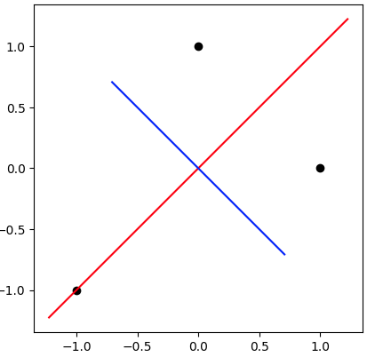
results in the eigenvector \mathbf{v} = [1,1]^\mathsf{T}, which is the first principal component.
For \lambda=1, solving the system results in the eigenvector \mathbf{v} = [1,-1]^\mathsf{T}, the second principal component.
The centered data and the principal components look like this: