The Normal distribution
Last time we discussed the idea of a continuous distribution with the uniform distribution as the central example. We also briefly met the normal distribution, which is our main example today.
This is all in section 4.1 of our text.
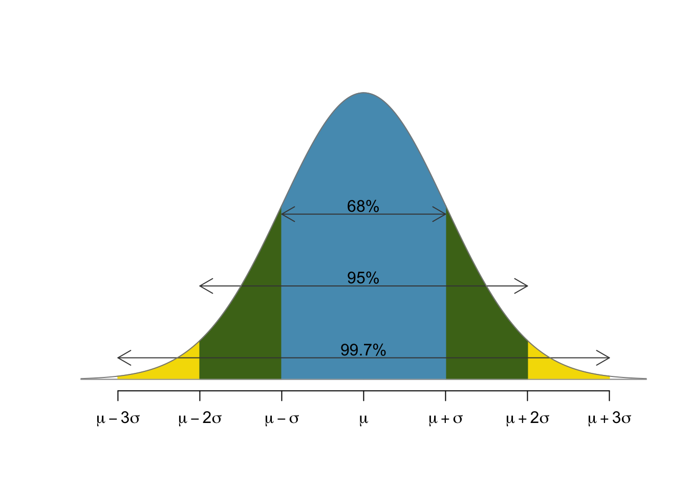
The 68-95-99.7
The previous picture arises by thinking about how the general normal relates to the to the standard normal. The basic rule of thumb is the 68-95-99.7 rule that states that
- 68% of the population lies within 1 standard deviation of the mean,
- 95% of the population lies within 2 standard deviations of the mean, and
- 99.7% of the population lies within 3 standard deviations of the mean.
This is true for the standard normal by direct computation and extends to all normal distributions through...
The Z-Score
Here's another way to think about it that will useful as we move to trickier examples. Recall that, if $X$ is normally distributed with mean $\mu$ and standard deviation $\sigma$, then we can translate $X$ to a standard normal via
$$ Z = \frac{X-\mu}{\sigma}. $$Computing this for a specific value of $X$ results in the $Z$-score for that value.
SAT example (again)
Recall that scores on the SAT exam are, by design, normally distributed with mean 500 and standard deviation 100.
Using that fact, at what percentile is a score or 700? That is, if we score a 700 on the SAT, then what percentage of folks can we expect scored below our score?
Solution 1
The first observation is that $$700 = 500 + 2\times100 = \mu+2\sigma.$$ That is, 700 is two standard deviations past the mean.
Now, our rules of thumb tell us that $95\%$ of the population lies within two standard deviations of the mean and only $5\%$ outside of that. Of that $5\%$, only half (or $2.5\%$) scored higher than us and the other $2.5\%$ scored far lower.
Thus, our 700 puts us at the $97.5^{\text{th}}$ percentile.
Solution 2
Alternatively, we can compute the $z$-score:
$$ Z = \frac{X-\mu}{\sigma} = \frac{700-500}{100} = 2. $$Note that the $2$ that comes out of this computation is exactly how many standard deviations past the normal the score off $700$ is. And, again, from our rules of thumb, it looks like $2.5\%$ of the students score.
The picture
The picture below illustrates the standard normal and the SAT normal for this problem.
If you're thinking those are the same picture with different numbers, then you're exactly right - that's the point!
But...
What if we want to know the percentile of a 672?
I guess the $Z$-score is
$$\frac{672-500}{100} = 1.72.$$So, how do we interpret that??
One Answer: Use a normal table.
Standard questions
Suppose that $Z$ is a random variable that has a standard, normal distribution. Then find
- $P(0<Z<1.5)$
- $P(Z>1.5)$
- $P(-1.23 < Z < 2.31)$
- The value $z_0$ of $Z$ for which $$P(0 < Z < z_0)=0.25.$$
Again, use a normal table.
A normal example
Suppose that $X$ is a normally distributed random variable with mean $\mu=17.5$ and standard devation $\sigma=3.9$. Then find $P(12.3<X<25.1)$.
Part of the solution: Note that the $Z$-score of $X=12.3$ is $$\frac{12.3-17.5}{3.9} \approx -1.33$$ and that the $Z$-score of $X=25.1$ is $$\frac{25.1-17.5}{3.9} \approx 1.95.$$ Thus, this is equivalent to asking for $$P(-1.33 < Z < 1.95).$$
We finish the problem using our normal table.
A data based example
Recall that our CDC data seems to imply that height is normally distribued with a mean of $67.18$ inches and a standard deviation of $4.12$. Suppose we pick a person at random. What is the probability that they are taller than $72$ inches?
Part of the solution: Note that the $Z$-score of $X=72$ is $$\frac{72-67.18}{4.12} \approx 1.17$$ We again finish the problem using our normal table.
Binomial relationship
Suppose we flip a coin 99 times. What is the probability that we get fewer than 47 heads?
Binomial solution
$$ \sum_{k=0}^{46} \begin{pmatrix}99\\k\end{pmatrix} 2^{99} \approx 0.273 $$That type of sum can be computed on the computer.
I wouldn't worry about that too much.
Normal solution
Alternatively, the mean of one coin flip is $1/2$ and its variance is
$$ p(1-p) = \frac{1}{2}\frac{1}{2} = \frac{1}{4} $$so that its standard deviation is also $1/2$. Thus, mean and standard deviation of 99 flips are $99/2$ and $\sqrt{99}/2$. This means that we can model the problem with a normal distribution and ask for $$ P(X<46.5) $$ where $X$ is normally distributed with mean $99/2$ and $\sqrt{99}/2$. Computing a $Z$ score, we get $Z=-0.603$. Looking this up in our normal table we get about the same answer.
Why Normal?
Why do we care so much about normal distributions?
Because of the Central Limit Theorem, of course!!
The central limit theorem
The central limit theorem is the theoretical explanation of why the normal distribution appears as the limit of binomials above and, therefore, so often in practice. Suppose that $X$ is a random variable which we evaluate a bunch of times to produce a sequence of numbers: $$X_1, X_2, \ldots, X_n.$$ We then compute the average of those values to produce a new value $\bar{X}$ defined by $$\bar{X} = \frac{X_1 + X_2 + \cdots + X_n}{n}.$$ The central limit theorem asserts that the random variable $\bar{X}$ is normally distributed. Furthermore, if $X$ has mean $\mu$ and standard deviation $\sigma$, then the mean and standard deviation of $\bar X$ are $\mu$ and $\sigma/\sqrt{n}$.
Note that all of this is true regardless of the distribution of $X$!
Binomials and Normals
The interactive tool below allows you to play with the parameters defining a binomial distribution and shows how the corresponding normal fits in.
