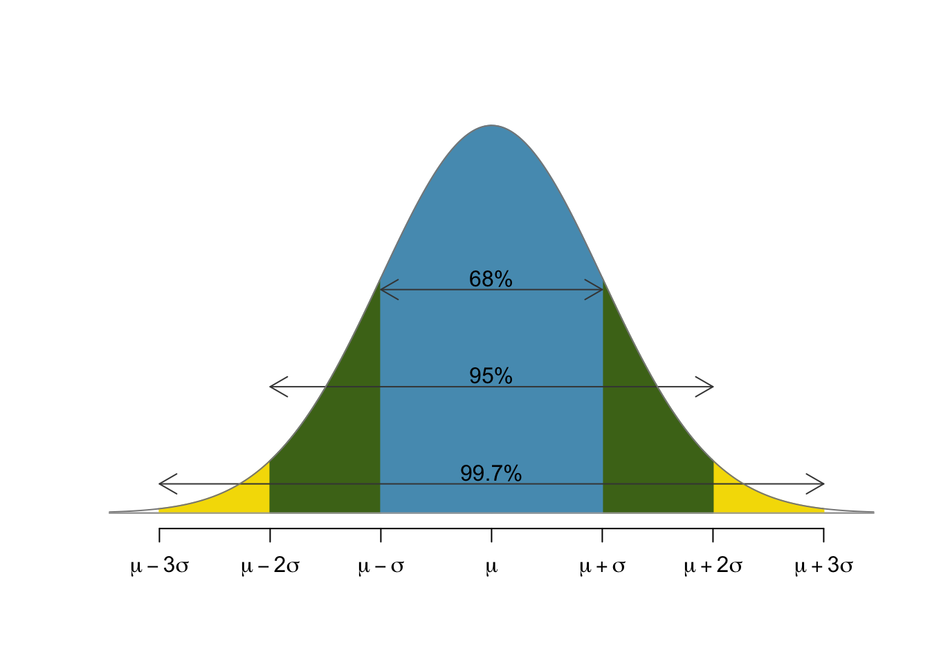
More normal

Today, we'll learn more about the normal distribution and see a tool that's great for ensuring that you get enough precision for your homework answers.

Recap

We've learned a lot over the couple of days about the normal distribution:

Computing with the normal

Key question now is - given a normally distributed random variable $X$ with mean $\mu$ and standard deviation $\sigma$, how do we compute quantities like

\begin{align} &P(X < x_0), \text{ or} \\ &P(X > x_0), \text{ or} \\ &P(x_1< X < x_0) \end{align}

Last time we learned how to do this using our normal table. Today, we'll learn how to use a more flexible and precise tool on the computer.

Example

Suppose that $X$ is normally distributed with mean $42.3$ and standard deviation $3.4$. Compute,

\begin{align} &P(X < 45), \\ &P(X > 45), \text{ and} \\ &P(40 < X < 45) \end{align}

Step 1: The first step is the same as before - we compute the $Z$-scores for the values $40$ and $45$. Once we have the $Z$-scores, we can compute those values to the standard normal distribution. Recall that the formula for a $Z$-score is

$$Z = \frac{X-\mu}{\sigma}.$$

Thus, for this example we have

$$z_1 = \frac{40-42.3}{3.4} = -0.67647 \: \text{ and } \: z_2 = \frac{45-42.3}{3.4} = 0.79412.$$

Example (cont)

For Step 2, we just plug the $Z$-score into the simple calculator below. We've got a more detailed version on our class webpage.

Data

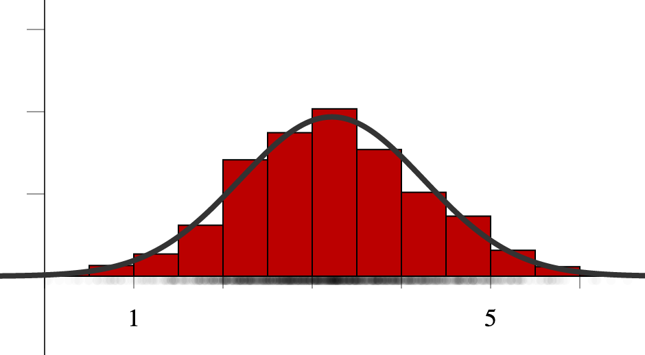
Of course, our driving mission is to understand data, be it categorical or numerical. Don't forget that data drives the following histogram, that in turn drives the approximating normal curve.

Example

Suppose that NBA players have an average height of $6.5277$ feet with a standard deviation of $0.285$ feet. Supposing their heights are normally distributed, find the proportion of NBA players taller than $6'9''$.

Solution: First, let's express $6'9''$ in terms of feet: $$6'9'' = \left(6 +9/12\right)\text{ ft} = 6.75 \text{ ft}.$$ We then compute the $Z$-score:

$$Z = \frac{6.75 - 6.5277}{0.285} = 0.78.$$

Finally, we plug that number into our calculator to get $$P(Z<0.78)\approx0.782305.$$ Thus, our answer is $1-0.782305 = 0.21769$.

Why Normal?

Why do we care so much about normal distributions?

Because of the Central Limit Theorem, of course!!

The central limit theorem

The central limit theorem is the theoretical explanation of why the normal distribution appears as the limit of binomials above and, therefore, so often in practice. Suppose that $X$ is a random variable which we evaluate a bunch of times to produce a sequence of numbers: $$X_1, X_2, \ldots, X_n.$$ We then compute the average of those values to produce a new value $\bar{X}$ defined by $$\bar{X} = \frac{X_1 + X_2 + \cdots + X_n}{n}.$$ The central limit theorem asserts that the random variable $\bar{X}$ is normally distributed. Furthermore, if $X$ has mean $\mu$ and standard deviation $\sigma$, then the mean and standard deviation of $\bar X$ are $\mu$ and $\sigma/\sqrt{n}$.

Note that all of this is true regardless of the distribution of $X$!

Binomials and Normals

The interactive tool below allows you to play with the parameters defining a binomial distribution and shows how the corresponding normal fits in.

Modeling numerical and categorical data

Here's an interactive illustration of how a Normal distribution models data:

Data driven

Note that the image is data driven. That is,

• The data comes first,
• then comes the histogram for the data,
• and finally, the curve that models data.

More specifically, the curve on the previous slide is the normal curve whose mean and standard deviation is the same as the data.