The Normal distribution
Last time we discussed the idea of a continuous distribution with the uniform distribution as the central example. We also briefly met the normal distribution, which is our main example today.
This is all in section 4.1 of our text.
Motivating example (again)
Suppose we go outside, grab the first person we see and measure their height. Accoring the data in our CDC data set, the average person has a height of about 67.18 inches. I suppose that our randomly grabbed person will have a height of close to that 67.18 inches. In fact, most people have a height of $$67.18 \pm 4 \text{ inches}.$$ Of course, there are people taller than 72 inches and shorter than 62 inches, but the number of folks you find of a certain height grows more sparse as we move away from the mean.
A normal density function
If we try to plot a curve that meets the criteria of a density function for heights, I guess it might look something like so:

Note that the area is concentrated near the mean of $67.18$. The shaded area represents 1 standard deviation (or $4.12$) away from the mean; which represents about $68\%$ of the population. There are people 2 and even 3 standard deviations away from the mean but they taper off rapidly.
The family of normal distributions
There's more than one normal distribution; there's a whole family of them - each specified by a mean and standard deviation.
All normal distributions have the same basic bell shape and the area under every normal distribution is one.
The mean $\mu$ of a normal distribution tells you where its maximum is.
The standard deviation $\sigma$ of a normal distribution tells you how concentrated it is about its mean.
The standard normal distribution is the specific normal with mean $\mu=0$ and standard deviation $\sigma=1$.
The family album
The interactive graphic below shows how the mean and standard deviation determine the corresponding normal distribution.
Standardizing normals
Any normally distributed random variable $X$ (with mean $\mu$ and standard deviation $\sigma$) can be translated to the standard normal $Z$ via the formula
$$Z = \frac{X-\mu}{\sigma}.$$Given a normally distributed random variable $X$ that obtains the value $x$, the computation
$$z = \frac{x-\mu}{\sigma}$$is called the $Z$-score for $x$.
The behavior of the standard normal
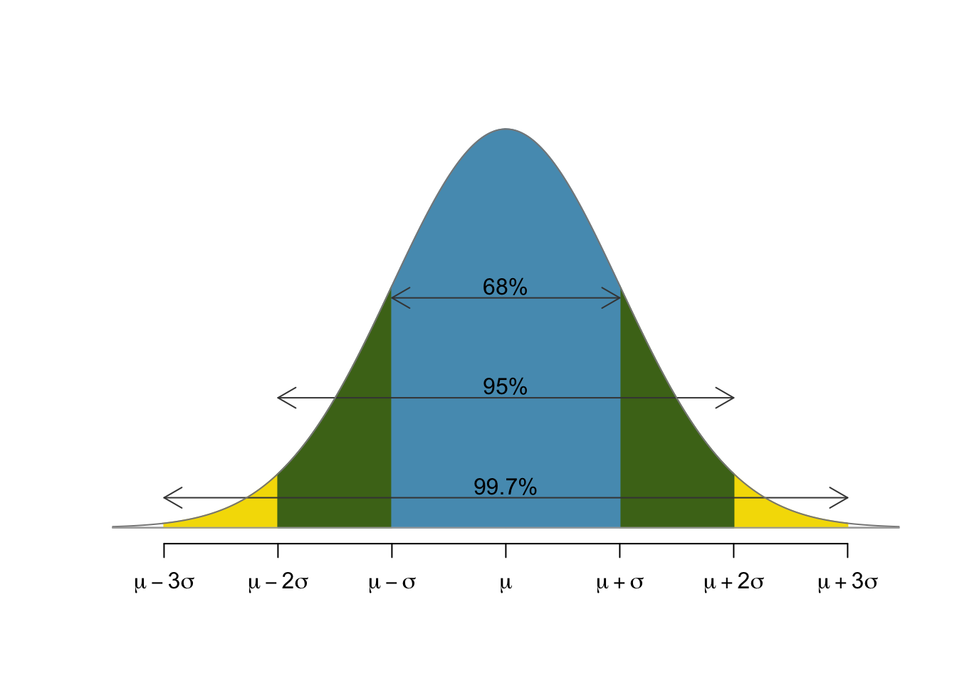
Since we can relate any normally distributed random variable to the standard normal, it's of great interest to fully understand the standard normal. There is a statistical rule of thumb for this purpose called the 68-95-99.7 rule that states that
- 68% of the population lies within 1 standard deviation of the mean,
- 95% of the population lies within 2 standard deviations of the mean, and
- 99.7% of the population lies within 3 standard deviations of the mean.
A picture of the standard behavior
Example
Let's suppose that the mean life expectancy of a cat is 14 years with a standard deviation of 2.5 years. Assuming that the cats' life spans are normally distributed, is it reasonable to expect a cat to live to 22 years old?
Solution: Well, the $z$-score for a 22 year old kitty cat would be $$Z = \frac{22-14}{2.5} = 3.2.$$ As we know, only $0.3\%$ of cats live beyond a $z$-score of 3, so a 22 year old cat would be quite rare indeed.
Another example
Scores on the SAT exam are, by design, normally distributed with mean 500 and standard deviation 100.
Using that fact, at what percentile is a score or 700? That is, if we score a 700 on the SAT, then what percentage of folks can we expect scored below our score?
Solution
The first observation is that $$700 = 500 + 2\times100 = \mu+2\sigma.$$ That is, 700 is two standard deviations past the mean.
Now, our rules of thumb tell us that $95\%$ of the population lies within two standard deviations of the mean and only $5\%$ outside of that. Of that $5\%$, only half (or $2.5\%$) scored higher than us and the other $2.5\%$ scored far lower.
Thus, our 700 puts us at the $97.5^{\text{th}}$ percentile.
The Z-Score
Here's another way to think about it that will useful as we move to trickier examples. Recall that, if $X$ is normally distributed with mean $\mu$ and standard deviation $\sigma$, then we can translate $X$ to a standard normal via
$$ Z = \frac{X-\mu}{\sigma}. $$Computing this for a specific value of $X$ results in the $Z$-score for that value.
For the SAT example, the $Z$-score of 700 given $\mu=500$ and $\sigma=100$ is
$$ Z = \frac{700-500}{100} = 2. $$Furthermore, the area under the standard normal to the left of 2 is about $0.975$.
The picture
The picture below illustrates the standard normal and the SAT normal for this problem.

If you're thinking those are the same picture with different numbers, then you're exactly right - that's the point!
But...
What if we want to know the percentile of a 672?
I guess the $Z$-score is
$$\frac{672-500}{100} = 1.72.$$So, how do we interpret that??
One Answer: Use a normal table.
Standard questions
Suppose that $Z$ is a random variable that has a standard, normal distribution. Then find
- $P(0<Z<1.5)$
- $P(Z>1.5)$
- $P(-1.23 < Z < 2.31)$
- The value $z_0$ of $Z$ for which $$P(0 < Z < z_0)=0.25.$$
A normal example
Suppose that $X$ is a normally distributed random variable with mean $\mu=17.5$ and standard devation $\sigma=3.9$. Then find $P(12.3<X<25.1)$.
Part of the solution: Note that the $Z$-score of $X=12.3$ is $$\frac{12.3-17.5}{3.9} \approx -1.33$$ and that the $Z$-score of $X=25.1$ is $$\frac{25.1-17.5}{3.9} \approx 1.95.$$ Thus, this is equivalent to asking for $$P(-1.33 < Z < 1.95).$$
We finish the problem using our normal table.
A data based example
Recall that our CDC data seems to imply that height is normally distribued with a mean of $67.18$ inches and a standard deviation of $4.12$. Suppose we pick a person at random. What is the probability that they are taller than $72$ inches?
Part of the solution: Note that the $Z$-score of $X=72$ is $$\frac{72-67.18}{4.12} \approx 1.17$$ We again finish the problem using our normal table.