Power Iteration
Today, we're going to talk about powers of matrices and how that leads to a way to compute the dominant eigenvector of a matrix.
Intro code
Can you see what's interesting about the following code?
								from numpy.random import rand,seed
								from scipy.linalg import norm

								M = rand(5,5)
								v = rand(5)
								for i in range(20):
								    v = M.dot(v)
								    v = v/norm(v)
								print(M.dot(v)/v)
								print(v)

								# Slightly simplified output:
								# [2.113 2.113 2.113 2.113 2.113]
								# [0.276 0.355 0.357 0.345 0.741]
Intro code (cont)
- That penultimate line
print(M.dot(v)/v)takes the vector $M\,\vec{v}$ and divides term-wise by $\vec{v}$. The result is vector of length 5 whose value is $2.113$ in each component. - Thus, $M\,\vec{v}=2.113\,\vec{v}$. That is, $\lambda=2.113$ is an eigenvalue of the matrix!
- The vector $\vec{v}$ itself is the corresponding eigenvector that we print in the last line.
- You can try it with live code. You should find that the process always converges to an eigenvalue/eigenvector pair.
Intro code (cont 2)
- This technique just illustrated is called the power method.
- While it doesn't always work, there is a surprisingly broad class of problems where it finds the so-called dominant eigenvector.
- It is the basis for Google's original pagerank algorithm.
- Our main objective today is to understand when and why the power method might work.
Iteration
The basic idea behind iteration is very simple and quite broad.
- Given: a function $f$ mapping a set $S$ to itself and a point $x_0 \in S$.
- Let $x_1=f(x_0)$,
- $x_2=f(x_1),\, \ldots$
- $x_n=f(x_{n-1})$.
- This recursively defines an infinite sequence of values $(x_k)_{k=1}^{\infty}$.
- Another way to write the $k^{\text{th}}$ value is $x_k=f^k(x_0)$.
Iteration example
Let $f(x) = \frac{1}{2}x$ and let $x_0=12$. Then our sequence is
$$\left\{12,6,3,\frac{3}{2},\frac{3}{4},\frac{3}{8},\frac{3}{16},\frac{3}{32}\right\}.$$- Note that each value is $\frac{1}{2}\times\text{ the previous value}$.
- It's pretty easy to see that the sequence converges to zero.
- In fact, the $k^{\text{th}}$ value is $\frac{1}{2^{k}}\times12$.
More generally, if $a\in\mathbb R$, we define $f(x)=ax$ and let $x_0\in\mathbb R$, then $f^{k}(x_0)=a^kx_0$.
Matrix iteration
Iteration via multiplication by a matrix is very similar:
- Given: a matrix $A\in\mathbb R^{n\times n}$ and a vector $\vec{v}_{(0)}\in\mathbb R^n$
- Define $\vec{v}_{(k)}$ recursively by $\vec{v}_{(k)} = A\,\vec{v}_{(k-1)}$
- Then $\vec{v}_{(k)} = A^k\,\vec{v}_{(0)}$.
Note that we've used parentheses to distinguish the terms of our sequence from our growing list of sub-scripts and super-scripts.
Matrix iteration example
The image below explores the iteration of $\vec{v} \to T\,\vec{v}$, where
$$T = \frac{1}{5}\begin{pmatrix}3&1\\1&3\end{pmatrix}.$$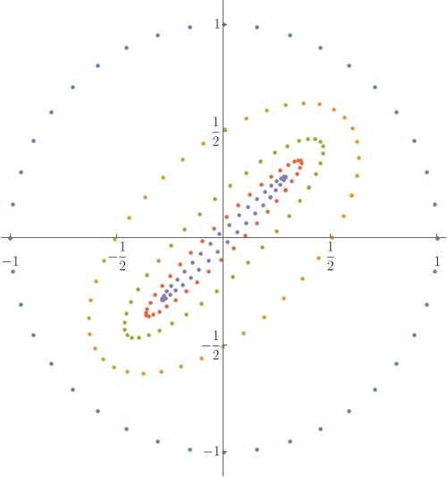
The outer ring is a set of initial seeds and each subsequent smaller ring is the image under multiplication by $T$ of the previous ring.
Iteration and eigenstructure
We'll explain why iteration should converge to an eigenvector under the following assumptions:
-
Suppose $A\in\mathbb R^{n\times n}$ is complete.
(That is, $A$ has $n$ linearly independent eigenvectors $\vec{u}_1,\vec{u}_2,\ldots,\vec{u}_n$ that necessarily form a basis for $\mathbb C^n$.) -
Suppose also, that $A$ has a single eigenvalue that is larger in absolute value than all the other eigenvalues. We will call this the dominant eigenvalue and will assume that it is $\lambda_1$ in the list of eigenvalues $(\lambda_k)$.
(Since complex eigenvalues come in conjugate pairs, this implies that this dominant eigenvalue is real.)
Iteration and eigenstructure (cont)
- Start with $\vec{v}_{(0)}\in\mathbb R^n$ chosen essentially randomly.
- Write $\vec{v}_{(0)}$ can be written as a linear combination of the eigenvectors of $A$: $$\vec{v}_{(0)} = c_1 \vec{u}_1 + c_2 \vec{u}_2 + \cdots + \vec{u}_n.$$
- Then, by linearity, $$A^k \vec{v}_{(0)} = c_1 \lambda_1^k \vec{u}_1 + c_2 \lambda_2^k \vec{u}_2 + \cdots + \lambda_n^k \vec{u}_n.$$
- Thus, $$\frac{1}{\lambda_1^k}A^k \vec{v}_{(0)} = c_1 \vec{u}_1 + c_2 \left(\frac{\lambda_2}{\lambda_1}\right)^k \vec{u}_2 + \cdots + \left(\frac{\lambda_n}{\lambda_1}\right)^k \vec{u}_n \to c_1\,\vec{u}_1.$$
Iteration and eigenstructure (cont 2)
- In practice, we don't know $\lambda_1$ as we apply the algorithm. Thus, we simply normalize the vector at each step.
- While not every matrix has a dominant eigenvalue, there are many important applications where a dominant eigenvalue is guaranteed.
-
The most general theorem guaranteeing a dominant eigenvalue is the Perron-Frobenius theorem that we discussed when we first met EigenRanking:
If the square matrix $A$ has nonnegative entries, then it has an eigenvector $\vec{r}$ with nonnegative entries corresponding to a positive eigenvalue $\lambda$. If $A$ is irreducible, then $\vec{r}$ has strictly positive entries, is unique, simple, and the corresponding eigenvalue is the one of largest absolute value.
Iteration and eigenstructure (cont 3)
The eigenstructure clarifies the iterative process.
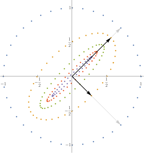
- Compute eigenstructure using
eigorthe power method. - It's the same matrix we examined before.
- Faint arrows are eigenvectors; dark arrows are their images.
Sparse matrices
-
A sparse matrix is one with a lot of zeros.
- Example: Google's Pagerank Matrix
- On a computer, we can represent a sparse matrix by indicating the positions and values of the non-zero entries.
- We can also multiply sparse matrices very quickly.
- The power method is particularly well suited to applications where sparse matrices arise.
Simple example
The following matrix can be stored with 27 integers as a sparse matrix, versus 100 integers as a full matrix.
$$\begin{pmatrix} \color{lightgray}0 & 1 & \color{lightgray}0 & \color{lightgray}0 & \color{lightgray}0 & \color{lightgray}0 & \color{lightgray}0 & \color{lightgray}0 & \color{lightgray}0 & \color{lightgray}0 \\ \color{lightgray}0 & \color{lightgray}0 & 2 & \color{lightgray}0 & \color{lightgray}0 & \color{lightgray}0 & \color{lightgray}0 & \color{lightgray}0 & \color{lightgray}0 & \color{lightgray}0 \\ \color{lightgray}0 & \color{lightgray}0 & \color{lightgray}0 & 3 & \color{lightgray}0 & \color{lightgray}0 & \color{lightgray}0 & \color{lightgray}0 & \color{lightgray}0 & \color{lightgray}0 \\ \color{lightgray}0 & \color{lightgray}0 & \color{lightgray}0 & \color{lightgray}0 & 4 & \color{lightgray}0 & \color{lightgray}0 & \color{lightgray}0 & \color{lightgray}0 & \color{lightgray}0 \\ \color{lightgray}0 & \color{lightgray}0 & \color{lightgray}0 & \color{lightgray}0 & \color{lightgray}0 & 5 & \color{lightgray}0 & \color{lightgray}0 & \color{lightgray}0 & \color{lightgray}0 \\ \color{lightgray}0 & \color{lightgray}0 & \color{lightgray}0 & \color{lightgray}0 & \color{lightgray}0 & \color{lightgray}0 & 6 & \color{lightgray}0 & \color{lightgray}0 & \color{lightgray}0 \\ \color{lightgray}0 & \color{lightgray}0 & \color{lightgray}0 & \color{lightgray}0 & \color{lightgray}0 & \color{lightgray}0 & \color{lightgray}0 & 7 & \color{lightgray}0 & \color{lightgray}0 \\ \color{lightgray}0 & \color{lightgray}0 & \color{lightgray}0 & \color{lightgray}0 & \color{lightgray}0 & \color{lightgray}0 & \color{lightgray}0 & \color{lightgray}0 & 8 & \color{lightgray}0 \\ \color{lightgray}0 & \color{lightgray}0 & \color{lightgray}0 & \color{lightgray}0 & \color{lightgray}0 & \color{lightgray}0 & \color{lightgray}0 & \color{lightgray}0 & \color{lightgray}0 & 9 \\ \color{lightgray}0 & \color{lightgray}0 & \color{lightgray}0 & \color{lightgray}0 & \color{lightgray}0 & \color{lightgray}0 & \color{lightgray}0 & \color{lightgray}0 & \color{lightgray}0 & \color{lightgray}0 \end{pmatrix}$$Simple example (cont)
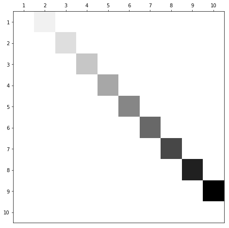
A visualization of the simple example: Zeros are white, the largest value is black, and intermediate values are gray.
Deeper example
- There are 353 NCAA basketball teams in division 1 and, prior to the COVID shutdown, those teams played a total of 5328 games.
- If we want to rank those teams using the eigen-ranking strategy we learned earlier, we need a $353\times353$ matrix. In row $i$ and column $j$ we might place the number of times that team $i$ defeated team $j$.
- To represent this as a dense matrix, we would need to store $353^2 = 124609$ entries.
- As a sparse matrix, we need only $4406$ entries. We also need to store their postitions for a total of $3\times4406=13218$ numbers that need to be stored.
Deeper example (cont)
A visualization of the NCAA basketball matrix is far too large to write down here but it's not hard to visualize:
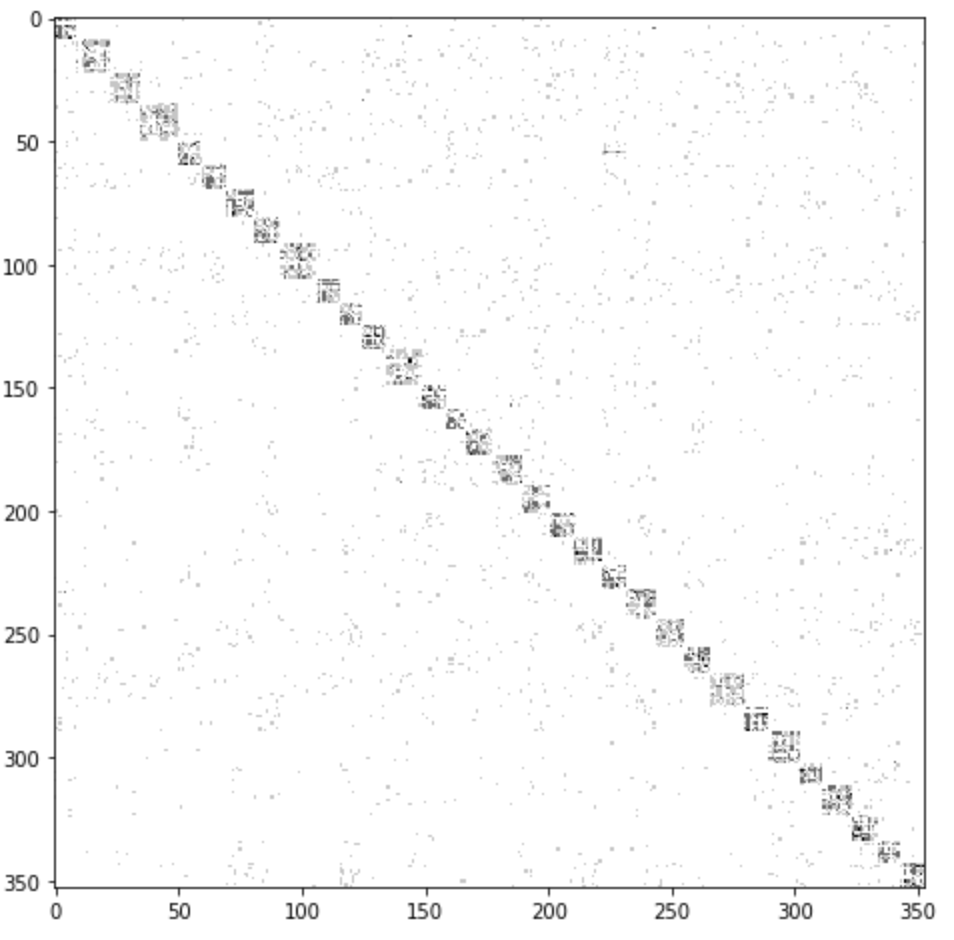
Clusters form on the diagonal because the teams are sorted into conferences.
Deeper example (cont 2)
scipy.sparse has a command called eigs designed to compute a few eigenvalue/eigenvector pairs of sparse matrices. Using that, I obtained the following strengths and rankings:
| Team | Strength |
|---|---|
| Florida_St | 0.150725 |
| Kansas | 0.150592 |
| Duke | 0.148579 |
| Villanova | 0.146498 |
| Maryland | 0.140609 |
| Michigan_St | 0.138507 |
| Baylor | 0.138496 |
| Creighton | 0.137279 |
| Oregon | 0.135733 |
| Louisville | 0.134360 |
| Virginia | 0.133454 |
| Kentucky | 0.129268 |
Other eigenvalues
- Inversion to find the smallest eigenvalue.
- Deflation to find the second largest eigenvalue.
- Shifting to find an eigenvalue near a suspected location
A working example
We're going to run through some computations with the following matrix:
$$ M = \left( \begin{array}{ccccc} 548 & -692 & 44 & 378 & 184 \\ 212 & -268 & 16 & 148 & 68 \\ 100 & -108 & -24 & 22 & -12 \\ -576 & 728 & -56 & -400 & -208 \\ 296 & -380 & 44 & 222 & 124 \\ \end{array} \right) $$Imports and definition
								import numpy as np
								from scipy.linalg import norm,\
								 lu_solve, lu_factor
								M = np.array([
								  [548, -692, 44, 378, 184],
								  [212, -268, 16, 148, 68],
								  [100, -108, -24,22, -12],
								  [-576, 728, -56, -400, -208],
								  [296, -380, 44, 222, 124]
								])
The largest eigenvalue
								v = [1,1,1,1,1]
								for i in range(50):
								    v = M.dot(v)
								    v = v/norm(v)
Another eigenvalue
								MM = M - (-36)*np.identity(5)
								v = [1,1,1,1,1]
								for i in range(100):
								    v = MM.dot(v)
								    v = v/norm(v)
If $(\lambda,\vec{v})$ is an eigenpair for $M$, then $$(M-\lambda I)\vec{v} = M\vec{v}-\lambda\vec{v} = \vec{0}.$$ Thus, iteration of $M-\lambda I$ should converge to some other eigenvector.
The smallest eigenvalue
								lu = lu_factor(M)
								v = [1,1,1,1,1]
								for i in range(100):
								    v = lu_solve(lu,v)
								    v = v/norm(v)
Since $1/\lambda$ is an eigenvalue of $M^{-1}$ when $\lambda$ is an eigenvalue of $M$.
The SciPy Sparse routines
SciPy has library for working with sparse matrices that I'll describe here soon.