Complex eigenvalues

Today, I'm going to talk about complex eigenvalues - how we deal with them algebraically, how we interpret them geometrically, and how they increase the scope and power of the diagonalization techniques that we learned in the last presentation.

Textbook sections

This stuff is a bit strewn out through the textbooks, as it includes examples with complex eigenvalues as it goes along. Here are a few examples of where you can find info in the text:

• Example 8.9 on page 412
• Proposition 8.10 on page 413
• Example 8.31 on page 430

Complex numbers

We will use some of the very basics of complex numbers. We'll need to know that a complex number has the form $a+bi$, where $a$ and $b$ are real numbers and $i$ denotes $\sqrt{-1}$.

We'll also need to know how complex numbers as solutions of quadratics.

Quadratic example

If we want to solve $x^2+x+1=0$, we can apply the quadratic formula to get

Matrix example

Let $A = \begin{pmatrix}0 & -1 \\ 1 & 0\end{pmatrix}$, then

The roots of the characteristic polynomial $\lambda^2+1$ are exactly $\pm i$.

Example (cont 1)

The two standard coordinate basis vectors rotate through the angle $90^{\circ}$ under multiplication by $A$ since

Example (cont 2)

This can be extended to any vector since

Example (cont 3)

Putting this all together, multiplication by $A=\begin{pmatrix}0 & -1 \\ 1 & 0\end{pmatrix}$ induces rotation through $90^{\circ}$.

Generalization

Rotation through any angle $\theta$ can be represented via multiplication by

Generalization (cont 1)

The reason is the same:

Thus, multiplication by $A_{\theta}$ rotates $\vec{\imath}$ and $\vec{\jmath}$ through the angle $\theta$ and (by linear extension) any vector.

Generalization (cont 2)

Let's check the eigenvalues of $A_{\theta}$:

Generalization (cont 3)

We can compute the roots of $\lambda^2 - 2\cos(\theta)\lambda + 1$ by applying the quadratic formula. We get:

The point

Complex eigenvalues indicate rotation!

Application

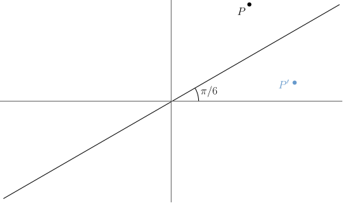
Given a line through the origin and a point $P$ not on the line, how can we describe the reflection $P'$ of that point?

Application (cont 1)

First note, that reflection across the $x$-axis is easy; it's just represented by

Thus, reflection across the line through the origin making the angle $\theta$ with the $x$-axis is represented by

Application (cont 2)

Rotation in 3D

We again start with an example:

Note that $M$ maps $\vec{\imath}\to\vec{\jmath}\to\vec{k}\to\vec{\imath}$.

Rotation in 3D (cont)

Since $M$ maps $\vec{\imath}\to\vec{\jmath}\to\vec{k}\to\vec{\imath}$, it's easy to imagine that it might represent rotation.

Rotation in 3D (cont 2)

So, what's the eigenstructure? If we compute the characteristic polynomial, we get:

Clearly, $\lambda=1$ is a root. You can solve $M\vec{v}=\vec{v}$ to show that $\langle 1,1,1 \rangle$ is a corresponding eigenvector. This represents the fixed direction around which the rotation happens.

Rotation in 3D (cont 3)

To find the other two roots, we factor:

The roots of that second factor are

Rotation in 3D (cont 4)

The fact that $\cos(2\pi/3)\pm i\sin(2\pi/3)$ are eigenvalues suggests that the matrix involves a rotation through the angle $2\pi/3$. To find the plane of rotation, we need the corresponding eigenvectors. Thus, we need to solve

Rotation in 3D (cont 5)

Taking the $+$ from the $\pm$, our system is equivalent to

Rotation in 3D (cont 6)

Allowing $z$ to be free and setting $z=1$, we obtain $x = -\frac{1}{2}-\frac{\sqrt{3}}{2} \text{ and } y = -\frac{1}{2}+\frac{\sqrt{3}}{2}$ so that an eigenvector is

Rotation in 3D (cont 7)

To interpret this, we could say that multiplication by $M$ fixes the line spanned by the vector $\langle 1,1,1 \rangle$ and rotates the plane spanned by the vectors $\langle -1/2,-1/2,1\rangle$ and $\langle -\sqrt{3}/{2}, \sqrt{3}/{2}, 0\rangle$.

3D action from eigenstructure

Generally, the situation can be a bit more complicated. Given a matrix $M\in\mathbb R^{3\times3}$, with one real eigenpair $(\lambda_r,\vec{v}_r)$ and two complex conjugate eigenpairs $(\lambda_{\pm},\vec{v}_{\pm})$,

• $\vec{v}_r$ spans a 1D subspace of $\mathbb R^3$ that is stretched or compressed according to $\lambda_r$
• The real and imaginary parts of $\vec{v}_{+}$ span a 2D subspace that is invariant of the action of $M$.

3D action from eigenstructure (cont)

• Note, though, that $\vec{v}_r$ need not be perpendicular to $\vec{v}_{\pm}$.
• Also, while the 2D subspace spanned by $\vec{v}_{\pm}$ will involve rotation, it need not be pure rotation; it might also involve scaling, reflection, or skewing.

Example

Here's a randomly generated example, like one that I'll ask you in the HW. We'll use the eigenstructure to deduce the geometric effect of the matrix

Example (cont)

Here's some Python code (and a live link) to compute the eigensystem:

from scipy.linalg import eig
M = [[2/3, -2/3, 2/3],
     [-2/3, -4/3, -4/3],
     [0, 5/3, -1/3]]
evals,evecs = eig(M)
print(evals)
print('---')
print(evecs)

# Output (slightly trimmed):
[  0.582]+0.j  -0.79+1.186j -0.79-1.186j]
---
[[-0.95+0.j  -0.37-0.065j -0.37+0.065j]
 [ 0.14+0.j  -0.20+0.52j  -0.20-0.52j]
 [ 0.26+0.j   0.73+0.j     0.73-0.j]]
				

Example (cont 2)

The first part of the output tells us the eigenvalues:

					[0.582+0.j  -0.791+1.186j -0.791-1.186j]
				

The js represent the imaginary unit; thus j**2==-1. Thus, we see one real eigenvalue, indicating a compression of about 0.58, and a pair of complex conjugate eigenvalues. As the magnitudes of those are larger than 1, we anticipate some expansion, as well as rotation.

Example (cont 3)

The next portion of the output is a matrix whose columns are the corresponding eigenvectors:

[[-0.95+0.j  -0.37-0.065j -0.37+0.065j]
 [ 0.14+0.j  -0.20+0.52j  -0.20-0.52j]
 [ 0.26+0.j   0.73+0.j     0.73-0.j]]
				

Note that the last two columns have non-zero imaginary parts and contain essentially the same information. We'll need to decompose one of those into real and imaginary parts.

Example (cont 4)

The middle column decomposes as

Those two vectors ($\langle -0.37, -0.2, 0.73 \rangle$ and $\langle - 0.065, 0.52, 0.73 \rangle$) span the subspace where the rotation happens.

Example (cont 5)

The image below illustrates. The black vectors come from the eigenstructure of the matrixand the red vectors are the images of those black vectors.

Diagonalization

As we move on, it will often be convenient to assume that a matrix is diagonalizable. Of course, not all matrices are diagonalizable but allowing the use of complex eigenvalues and eigenvectors greatly extends the class of matrices that are.

For example, a rotation matrix on $\mathbb R^2$ is certainly not diagonalizable since that would imply the existence of invariant 1D subspaces.

Diagonalization (cont)

As an example, you may feel free to verify the following by direct computation:

The matrices $S$ and $D$ above are chosen using eigenvalues and eigenvectors exactly we did before - they just have complex components.