Eigen-rankings
A basic example
Let's suppose that three competitors or teams (numbered zero, one, and two) compete against each other twice each in some type of contest - football, basketball, tiddly winks, what have you. How might we rank them based on the results that we see? For concreteness, suppose the results are the following:
- Team zero beat team one twice and team two once,
- Team one beat team two once,
- Team two beat team zero and team one once each.
We might represent this diagrammatically as follows:
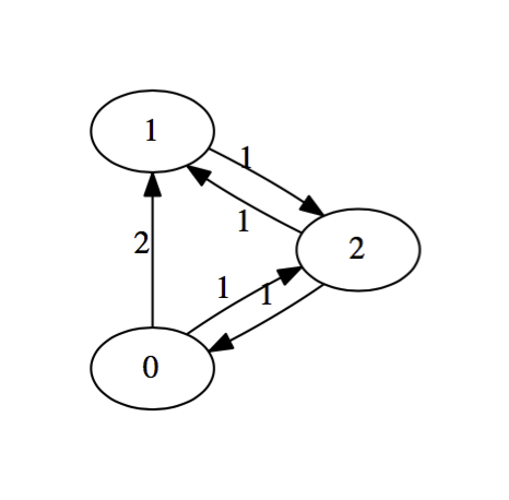
This configuration is called a directed graph or digraph. We construct it by placing an edge from team $i$ to team $j$ and labeling that edge with the number of times that team $i$ beat team $j$. We suppress zero edges. There an obvious matrix associated with a digraph called the adjacency matrix. The rows and column will be indexed by the teams. In row $i$ and column $j$, we place the label on the edge from team $i$ to team $j$. The adjacency matrix for this digraph is
$$\left(\begin{matrix} 0 & 2 & 1 \\ 0 & 0 & 1 \\ 1 & 1 & 0 \end{matrix}\right)$$It seems reasonably clear that team zero should be ranked the highest, having beaten both competitors a total of 3 times out of 4 possible tries. Team one, on the other hand won only 1 game out of it's four tries, while team two seems to be in the middle, having split it's game with both competitors. Certainly, the teams listed from worst to first should be: $1$, $2$, $0$.
Eigen-formulation
It turns out there's a lovely way to recover this exact ranking using the eigensystem of the adjacency matrix associated with the directed graph. The basic idea, together with some generalizations and improvements is described in The Perron-Frobenius Theorem and the Ranking of Football Teams by James Keener, though the idea dates back until at least the 1930s. The following outline follows Keener's most basic version.
Now, let's suppose we have $N$ participants in our collection of contests. We also suppose there is a vector $\vec{r}$ of rankings with positive entries $r_j$. Conceptually, $r_j$ represents the actual strength of the $j^{\text{th}}$ competitor. We wish to assign a positive score $s_i$ to each competitor. If competitor $i$ beats competitor $j$, we expect that to contribute positively to the score of competitor $i$. Furthermore, the stronger competitor $j$ was, the more we expect the contribution to be. Symbolically, we might write:
$$s_i = \frac{1}{n_i}\sum_{j=1}^N a_{ij}r_j.$$Thus, $s_i$ is a linear combination of the strengths of it's opponents. The normalization factor $n_i$ is the number of games that team $i$ played; we include it because we don't want a team's ranking to be higher simply because it played more games.
A key issue, of course, is how should the matrix of coefficients $A=(a_{ij})$ be chosen? Certainly, if team $i$ defeated team $j$ every time they played (there might be more than one contest between the two), then we expect $a_{ij}>0$. Beyond that, there's a lot of flexibility and the precise choice is one for experimentation and (hopefully) optimization. In the simple approach that follows, we'll take $a_{ij}$ to simply be the number of times that team $i$ defeated team $j$.
Finally, it seems reasonable to hope that our score $s_i$ of the $i^{\text{th}}$ team should be related to the actual strength $r_i$ of that team. Let's assume that they are, in fact, proportional: $\vec{s} = \lambda \vec{r}$. Put another way, we have $$A\vec{r} = \lambda\vec{r}.$$ That is, the actual ranking of strengths vector $\vec{r}$ is an eigen-vector of $A$!
The Perron-Frobenius theorem
At this point, we turn to some mathematical theory to guide us in our choice of eigenvector.
Theorem: If the square matrix $A$ has nonnegative entries, then it has an eigenvector $\vec{r}$ with nonnegative entries corresponding to a positive eigenvalue $\lambda$. If $A$ is irreducible, then $\vec{r}$ has strictly positive entries, is unique, simple, and the corresponding eigenvalue is the one of largest absolute value.
This all seems good because we certainly want a vector of positive rankings and the theorem tells us which one to choose. This eigenvalue/eigenvector pair is sometimes called dominant.
To some readers, the notion of an irreducible matrix is quite possibly new. There are a number of equivalent characterizations including:
- $A\vec{v}>0$, whenever $\vec{v}>0$,
- There is no permutation of the rows and columns of $A$ transforming the matrix into a block matrix of the form $$\left(\begin{matrix} A_{11} & A_{12} \\ 0 & A_{22} \end{matrix}\right),$$ where $A_{11}$ and $A_{22}$ are square.
- The associated digraph is strongly connected, i.e. there is a path from any vertex to any other.
I find the last characterization easiest to work with and it's easy to believe that it's likely to be satisfied, if teams play each other enough. Even if the matrix is not irreducible, the eigen-ranking approach can work. If not, it's often sufficient to work with the appropriate strongly connected component of the digraph.
The basic example revisited
Recall that the adjacency matrix associated with our simple example, written in code, is:
M = [
    [0,2,1],
    [0,0,1],
    [1,1,0]
]
According to the theory, this should have a unique positive eigenvalue whose magnitude is larger than the magnitude of any other eigenvalue. There should be an associated eigenvector with all positive entries. Of course, if $\vec{v}$ is an eigenvector, then so is $-\vec{v}$ (or any constant multiple). The theory tells us that we might as well just take the absolute value.
Here's the eigensystem for our simple example:
from scipy.linalg import eig
eig(M)
The result is a pair: a list of the eigenvalues and a matrix whose columns are the eigenvectors. Note that the last displayed eigenvalue, about $1.769$, has zero imaginary part and is clearly larger in absolute value than the other two, which are complex conjugates. The corresponding eigenvector has components all with the same sign. The absolute value of that eigenvector should be reasonable strengths associated with the teams, approximately: $$0.7235, \; 0.3396, \; 0.6009.$$ As expected, the zeroth team is the strongest, while the middle team is the weakest.
The B1G
The previous example was small enough to eyeball. Here's a real (so, more complicated) example: This past year's Big Ten regular football season. Since it's just the regular season, we're not including the championship game. Thus, each team played 8 games so we still don't have to worry about normalization. The visualization is bound to be messier, though. Here's an approach using a chord diagram.
Note that the width of the chord from team $i$ to team $j$ indicates how many points each team scored in that contest. The width varies so that it's proportional to points scored by each team at either endpoint. You can hover over the chords to get exact values. If we put those values in a matrix, we get:
import numpy as np
M = np.matrix([
    [0, 0, 10, 0, 25, 37, 17, 38, 10, 0, 0, 24, 38, 24],
    [0, 0, 0, 34, 14, 31, 0, 38, 34, 10, 27, 44, 35, 0],
    [19, 0, 0, 0, 3, 0, 23, 27, 20, 0, 12, 26, 30, 22],
    [0, 28, 0, 0, 7, 16, 10, 7, 0, 14, 0, 14, 48, 0],
    [42, 39, 10, 38, 0, 44, 0, 0, 0, 27, 21, 0, 52, 14],
    [34, 40, 0, 19, 10, 0, 0, 0, 31, 10, 7, 0, 27, 0],
    [40, 0, 19, 52, 0, 0, 0, 34, 38, 0, 31, 38, 42, 17],
    [42, 31, 24, 54, 0, 0, 7, 0, 13, 7, 0, 27, 0, 21],
    [29, 3, 0, 0, 0, 10, 22, 10, 0, 3, 0, 22, 0, 15],
    [0, 51, 0, 73, 56, 34, 0, 48, 52, 0, 28, 0, 56, 38],
    [0, 34, 17, 59, 28, 28, 26, 0, 0, 17, 0, 35, 27, 0],
    [6, 41, 20, 40, 0, 0, 31, 31, 24, 0, 7, 0, 0, 24],
    [10, 0, 0, 7, 0, 0, 7, 0, 0, 21, 6, 0, 0, 0],
    [23, 0, 24, 0, 35, 38, 38, 37, 24, 7, 0, 45, 0, 0]
])
The rows and columns of that matrix are indexed by the teams ordered alphabetically as follows:
b1g = [
    'Illinois','Indiana','Iowa','Maryland','Michigan',
    'Michigan State','Minnesota','Nebraska','Northwestern',
    'Ohio State','Penn State', 'Purdue', 'Rutgers', 'Wisconsin'
]
For example, Ohio State is the tenth team on that list and Michigan is fifth. Recalling that Python uses a zero-based indexing scheme, we should find the number of points that Ohio State scored against Michigan as follows:
M[9,4]
We now go through essentially the same process that we went through before.
vals, vecs = eig(M)
vals
Looks like the largest eigenvalue leads off the list in position zero. We're going to use a command called argsort to find out how to order the corresponding eigenvalue.
vec = abs(vecs[:,0])
ranking = np.argsort(vec).tolist()
ranking.reverse()
ranking
We then list the teams in that order:
[b1g[i] for i in ranking]
And their relative strengths, according to the eigenvector.
[vec[i] for i in ranking]
Not bad!