Intro to double integrals
Welcome to our first real online presentation! Today, I'm going to talk about double integrals.
The presentation works just like last time - use the arrows in the lower right to navigate through the slides and listen to the audio recording when the player appears (which it doesn't on this first slide).
Single variable integrals
Recall that the basic geometric question of single variable integration is - what is the area under a curve?
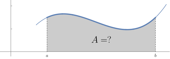
Approximating the area
We approximate the area using a collection of rectangles. The more rectangles; the better the approximation.
Riemann Sums
Add the (signed) areas to get the approximation
$$\text{Area under curve} \approx \sum_{i=1}^{n} f(x_i) \, \Delta x$$The definite integral
The limit as the Riemann sums as $n\to\infty$.
$$\int_a^b f(x) \, dx = \lim_{n\to\infty} \sum_{i=1}^{n} f(x_i) \, \Delta x$$Computing integrals
We generally compute integrals using either
- The Fundamental Theorem of Calculus: $$\int_a^b f(x) \, dx = F(b)-F(a)$$
- or numerical approximation
Applications
- Work
- Arc length
- Volumes of revolution, and...
- Volumes under surfaces!
Double integrals
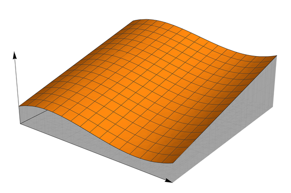
New motivating geometric question: Volume under a surface
Iterated integrals
If a function $f(x,y)$ is defined over a rectangular region $$[a,b]\times[c,d] = \{(x,y):a\leq x \leq b, c\leq y \leq d\},$$ Then it turns out we can get the exact volume under the graph of $f$ and over the rectangle using a so-called iterated integral: $$\int_c^d \int_a^b f(x,y) \, dx \, dy.$$
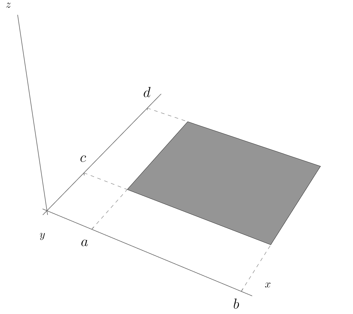
The domain
$$[a,b]\times[c,d] = \{(x,y):a\leq x \leq b, c\leq y \leq d\}$$is a rectangle in the domain of $f$.
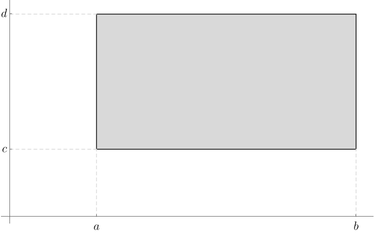
Bounds
Note that the bounds of the rectangle
$$[\color{red}a,\color{red}b]\times[\color{red}c,\color{red}d] = \{(x,y):\color{red}a\leq \color{green}x \leq \color{red}b, \color{red}c\leq \color{green}y \leq \color{red}d\}$$correspond to the bounds of integration
$$\int_{\color{red}c}^{\color{red}d} \int_{\color{red}a}^{\color{red}b} f(x,y) \, d\color{green}x \, d\color{green}y.$$The domain in space
The rectangle can be viewed in space, as well.
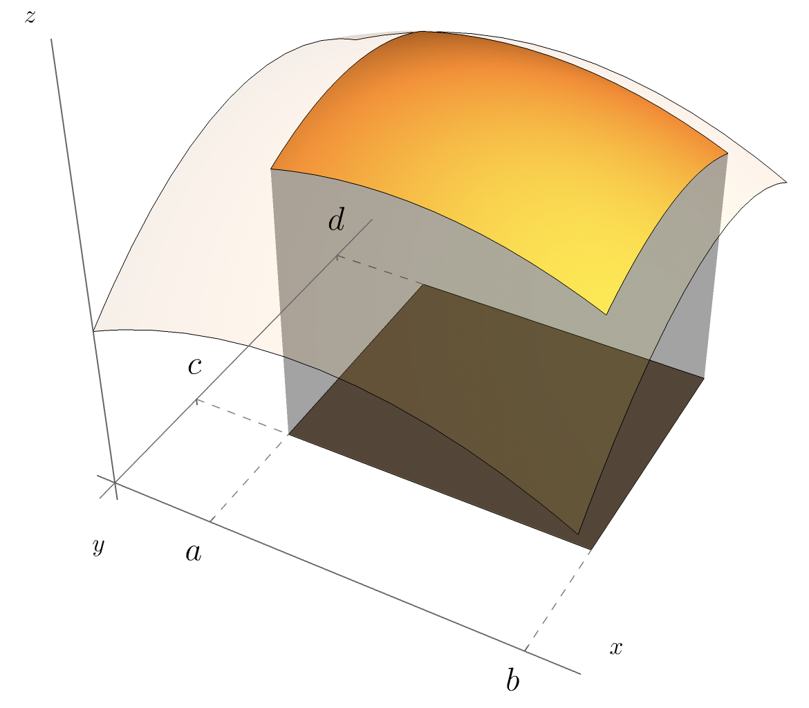
Domain with a plot
The integral represents the volume under a function and over the rectangle specified by the bounds of integration.
Example
Use an iterated integral to evaluate $$\int_0^2 \int_0^1 x y^3 \, dx \, dy$$ and interpret the result.
Interpretation
Again, the main point is that $$\int_0^2 \int_0^1 x y^3 \, dx \, dy$$ represents the (signed) volume under the graph of $f(x,y)=x y^3$ and over the rectangle $[0,1]\times[0,2]$.
Evaluation
We evalute the inner integral with respect to $x$, holding $y$ constant.
$$\begin{align*} \int_0^2 \color{red}{\int_0^1 x y^3 \, dx} \, dy &= \int_0^2 \color{red}{\frac{1}{2}x^2\bigg\rvert_0^1 y^3} dy \\ &= \frac{1}{2} \int_0^2 y^3 dy = \frac{1}{8}y^4 \bigg\rvert_0^2 = 2 \end{align*} $$Why's this work?
Given our motivating picture, why should the iterated integral strategy yield the volume under that surface?
Slicing
We approximate the volume by slicing it along the $y$ axis in slices of width $\Delta y$. Again, the more slices; the better the approximation.
Area under one slice
Now the cross-sectional area of the $i^{\text{th}}$ slice is $$A_i = \int_a^b f(x,y_i) dx.$$
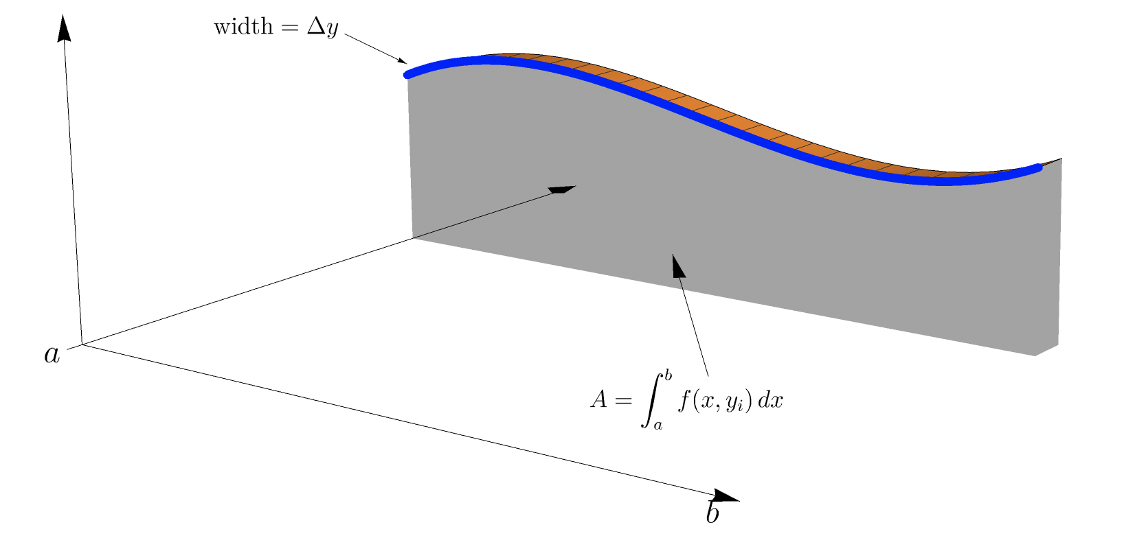
Volume of one slice
Since the we know the cross-sectional area of one slice and since it's width is $\Delta y$, it's volume is $$ \begin{align*} V_i &= \text{cross-sectional area} \times \Delta y \\ & = \int_a^b f(x,y_i) dx \times \Delta y. \end{align*} $$
Total volume
The total volume should be well approximated by the sum of the volumes of the slices. That sum is again a Riemann sum which should converge to an integral. $$ \begin{align*} V &= \sum_{i=1}^n \int_a^b f(x,y_i) dx \times \Delta y \\ &\to \int_c^d \int_a^b f(x,y) \, dx \, dy. \end{align*} $$