Modelling the $n$ body problem
%matplotlib inline
import matplotlib.pyplot as plt
import numpy as np
from scipy.integrate import odeint
The $n$-body problem asks: How do $n$ bodies in space that interact only through gravity behave? In this case, the total force acting on the $i^{\text{th}}$ body is the sum of the graviational forces from the other $n-1$ bodies. This total force induces an acceleration leading to the following equation for the $i^{\text{th}}$ body: $$m_i r_i'' = G m_i \sum_{j\neq i} \frac{r_j - r_i}{\|r_j-r_i\|^3}.$$ Note that $r$ is a vector indicating position. If we're working in the plane (as we will), then $r(t) = \langle x(t), y(t) \rangle$.
Of course, there are similar equations for other objects. This leads to $n$ second order equations for vector valued functions describing the motion. These may be translated to $2n$ second order equations involving $x$ and $y$ for planar motion or $3n$ second order equations involving $x$, $y$, and $z$ for motion in space. To express this as a first order system, we have twice as many equations.
We begin with a reasonably simple way to describe an initial configuration. Then we'll write code that automates the procedure of translating the initial configuration into a system of equations. Each object is described as a dictionary with mass m, position p, and velocity v keys. The initial condition is just a list of these.
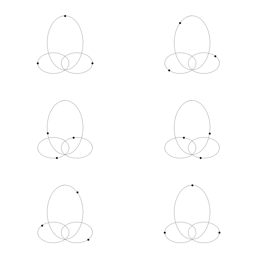
Our initial condition illustrates a fun stable configuration of three in celestial mechanics.
obj1 = {
    "m": 4,
    "p": (0,0),
    "v": (0,-1/np.sqrt(2))
}
obj2 = {
    "m": 4,
    "p": (1,0),
    "v": (0,1/np.sqrt(2))
}
obj3 = {
    "m": 0.0001,
    "p": (1/2,np.sqrt(3)/2),
    "v": (-np.sqrt(3/2),0)
}
init = [obj1,obj2,obj3]
To use SciPy's odeint , we'll need to write a function F(s,t) where s is a state vector and t is time. Of course, our system is autonomous so that t won't occur explicitly. When we have $n$ objects, our state vector will need $4n$ terms. The first $n$ terms will tell us the $x$ positions of our objects, the next $4n$ terms will tell us the $y$ positions of the objects, the third $4n$ terms will tell us the $x$ velocities of the objects, and the final $4n$ terms will tell us the $y$ velocities of the objects. Conceptually:
s looks like [xpos; ypos; xvel; yvel]
Where those components each have length $n$. I guess our update function F should then look like this:
F(s,t) looks like [xvel; yvel; xaccel; yaccel]
Of course, xaccel and yaccel need to be computed from the gravitational forces. Taking this all into account, I came up with something that looks like so:
G = 1
n = len(init)
def x_accel(s,i,j):
    m2 = init[j]['m']
    x1 = s[i]
    y1 = s[i+n]
    x2 = s[j]
    y2 = s[j+n]
    return m2*(x2-x1)/((x2-x1)**2 + (y2-y1)**2)**(3/2)
def y_accel(s,i,j):
    m2 = init[j]['m']
    x1 = s[i]
    y1 = s[i+n]
    x2 = s[j]
    y2 = s[j+n]
    return m2*(y2-y1)/((x2-x1)**2 + (y2-y1)**2)**(3/2)
def xpp(s,i):
    other_indices = list(range(n))
    other_indices.remove(i)
    return G*sum([x_accel(s,i,j) for j in other_indices])
def ypp(s,i):
    other_indices = list(range(n))
    other_indices.remove(i)
    return G*sum([y_accel(s,i,j) for j in other_indices])
def F(s,t):
    return np.concatenate(
        (s[2*n:3*n],s[3*n:4*n],
         [xpp(s,i) for i in range(n)],
         [ypp(s,i) for i in range(n)]))
To use it, we need an initial state vector $s$ with the form just described but corresponding to our initial conditions.
x0 = [o['p'][0] for o in init]
y0 = [o['p'][1] for o in init]
vx0 = [o['v'][0] for o in init]
vy0 = [o['v'][1] for o in init]
s0 = np.concatenate((x0,y0,vx0,vy0))
Then, we solve over some desired time interval.
t = np.linspace(0,2,1000)
solution = odeint(F,s0,t)
After a little experimentation I came up with the following pic function for visualization.
def pic(k=0):
    for i in range(n):
        plt.plot(solution[:,i], solution[:,n+i], 'gray', linewidth=0.5)
    for i in range(n):
        plt.plot(solution[k,i], solution[k,n+i], 'ko')
    ax = plt.gca()
    ax.set_aspect(1)
    ax.set_xlim(-0.1,1.1)
    ax.set_ylim(-0.2,1)
    plt.axis('off');
The generic picture looks like so:
pic(959)
And here it is in action:

The code should work with any list of n initial objects. It's not hard to write a reasonable random initiator. It should be understood, though, that a singularity will likely be hit, if the integration proceeds long enough.
import random
random.seed(2)
def random_object(): return {
        "m": random.random(),
        "p": (random.uniform(-2,2), random.uniform(-2,2)),
        "v": (0,0) # Could be set in principle, but zero total momentum is easy
    }
init = [random_object() for i in range(5)]
init
Here's a slightly different pic command.
def pic(k=0):
    for i in range(n):
        plt.plot(solution[0:k,i], solution[0:k,n+i], 'gray', linewidth=0.5)
    for i in range(n):
        plt.plot(solution[k,i], solution[k,n+i], 'ko')
    ax = plt.gca()
    ax.set_aspect(1)
    ax.set_xlim(-2,2)
    ax.set_ylim(-2,2)
    plt.axis('off');
Running again through the code above, we can generate an animation like so:
