First off, we focus on some parametrized family in complex iteration for the same reasons that we did so in the real case: Doing so facilitates the exploration of the range of possible behaviors that can arise in complex iteration. As it turns out, the introduction of parametrized families leads to fascinating mathematics in and of itself, like the bifurcation diagram in real iteration and its complex analog - the Mandelbrot set.
It's still fair to ask, though, “why this particular parametrized family”? As we've seen, the dynamics of first degree polynomials are quite simple; thus, it makes sense to move to at least quadratics. Furthermore, as it turns out, any quadratic is affinely conjugate to exactly one \(f_c\text{.}\) Note that by “affinely conjugate”, we mean that the conjugacy function has the form \(\varphi(z) = az+b\text{.}\) This statement is made more precise by the following two lemmas.
Lemma5.1.1
Let \(g(z) = \alpha z^2 + \beta z + \gamma\text{.}\) Then \(\varphi(z) = \alpha z + \beta/2\) conjugates \(f_c\) to \(g\) for
\begin{equation*}
c = \frac{1}{4}(2\beta - \beta^2 + 4\alpha\gamma).
\end{equation*}
More precisely, \(\varphi\circ g = f\circ\varphi\text{.}\)
Equating the coefficients of \(z^2\text{,}\) we see that \(a=0\) or \(a=1\text{.}\) Of course, \(a\) cannot be zero, or else \(\varphi\) is not a genuine affine function. Thus, \(a=1\text{.}\) Equating the coefficients of \(z\text{,}\) we see that \(2ab=0\text{,}\) thus \(b=0\text{.}\) Equating the constant terms and taking the now known values of \(a\) and \(b\) into account, we see that \(c_1=c_2\text{.}\)
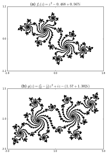
The significance of affine conjugation is illustrated in figure Figure 3. On the top, we see the Julia set of \(f_c(z)\) for \(c=-0.468+0.567i\text{.}\) On the bottom, we see the Julia set of
is an affine transformation which simply rotates, scales, and shifts the plane. In fact, the Julia set on the bottom is exactly the image of the Julia set on the top after an expansion by the factor 2, a rotation through the angle \(45^{\circ}\text{,}\) and a shift by the complex number \(1-i\text{.}\)