Eigen-Rankings
A basic example
Let's suppose that three competitors or teams (numbered zero, one, and two) compete against each other twice each. How might we rank them based on the results that we see? For concreteness, suppose the results are the following:
- Team zero beat team one twice and team two once,
- Team one beat team two once,
- Team two beat team zero and team one once each.
We might represent this diagrammatically as follows:
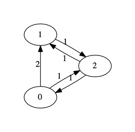
This configuration is called a directed graph or digraph. We construct it by placing an edge from team $i$ to team $j$ and labeling that edge with the number of times that team $i$ beat team $j$. We supress zero edges. There an obvious matrix associated with a digraph called the adjacency matrix. The rows and column will be indexed by the teams. In row $i$ and column $j$, we place the label on the edge from team $i$ to team $j$. The adjacency matrix for this digraph is
$$\left(\begin{matrix} 0 & 2 & 1 \\ 0 & 0 & 1 \\ 1 & 1 & 0 \end{matrix}\right)$$It seems reasonably clear that team zero should be ranked the highest, having beaten both competitors a total of 3 times out of 4 possible tries. Team one, on the other hand won only 1 game out of it's four tries, while team two seems to be in the middle, having split it's game with both competitors. Certainly, the teams listed from worst to first should be: $1$, $2$, $0$.
Eigen-formulation
It turns out there's a lovely way to get at this exact ranking using the eigensystem of the adjacency matrix associated with the directed graph. The basic idea, together with some generalizations and improvements is described in The Perron-Frobenius Theorem and the Ranking of Football Teams by James Keener, though the idea dates back until at least the 1930s. The following outline follows Keener's most basic version.
Now, let's suppose we have $N$ participants in a collection of contests - football, basketball, tiddly winks, what have you. We also suppose there is a vector $\vec{r}$ of rankings with positive entries $r_j$. Conceptually, $r_j$ represents the actual strength of the $j^{\text{th}}$ competitor. We wish to assign a positive score $s_i$ to each competitor. If competitor $i$ beats competitor $j$, we expect that to contribute positively to the score of competitor $i$. Furthermore, the stronger competitor $j$ was, the more we expect the contribution to be. Symbolically, we might write:
$$s_i = \frac{1}{n_i}\sum_{j=1}^N a_{ij}r_j.$$Thus, $s_i$ is a linear combination of the strengths of it's opponents. The normalization factor $n_i$ is the number of games that team $i$ played; we include it because we don't want a team's ranking to be higher simply because it played more games.
A key issue, of course, is how should the matrix of coefficients $A=(a_{ij})$ be chosen? Certainly, if team $i$ defeated team $j$ every time they played (there might be more than one contest between the two), then we expect $a_{ij}>0$. Beyond that, there's a lot of flexibility and the precise choice is one for experimentation and (hopefully) optimization. In the simple approach that follows, we'll take $a_{ij}$ to simply be the number of times that team $i$ defeated team $j$.
Finally, it seems reasonable to hope that our score $s_i$ of the $i^{\text{th}}$ team should be related to the actual strength $r_i$ of that team. Let's assume that they are, in fact, proportional: $\vec{s} = \lambda \vec{r}$. Put another way, we have $$A\vec{r} = \lambda\vec{r}.$$ That is, the actual ranking of strengths vector $\vec{r}$ is an eigen-vector of $A$!
The Perron-Frobenius theorem
At this point, we turn to some mathematical theory to guide us in our choice of eigenvector.
Theorem: If the square matrix $A$ has nonnegative entries, then it has an eigenvector $\vec{r}$ with nonnegative entries corresponding to a positive eigenvalue $\lambda$. If $A$ is irreducible, then $\vec{r}$ has strictly positive entries, is unique, simple, and the corresponding eigenvalue is the one of largest absolute value.
This all seems good because we certainly want a vector of positive rankings and the theorem tells us which one to choose. This eigenvalue/eigenvector pair is sometimes called dominant.
To some readers, the notion of an irreducible matrix is quite possibly new. There are a number of equivalent characterizations including:
- $A\vec{v}>0$, whenever $\vec{v}>0$,
- There is no permutation of the rows and columns of $A$ transforming the matrix into a block matrix of the form $$\left(\begin{matrix} A_{11} & A_{12} \\ 0 & A_{22} \end{matrix}\right),$$ where $A_{11}$ and $A_{22}$ are square.
- The associated digraph is strongly connected, i.e. there is a path from any vertex to any other.
I find the last characterization easiest to work with and it's easy to believe that it's likely to be satisfied, if teams play each other enough. Even if the matrix is not irreducible, the eigen-ranking approach can work. If not, it's often sufficient to work with the appropriate strongly connected component of the digraph.
The basic example revisited
Recall that the adjacency matrix associated with our simply example, written in code, is:
M = [
    [0,2,1],
    [0,0,1],
    [1,1,0]
]
According to the theory, this should have a unique positive eigenvalue whose magnitude is larger than the magnitude of any other eigenvalue. There should be an associated eigenvector with all positive entries. Of course, if $\vec{v}$ is an eigenvector, then so is $-\vec{v}$ (or any constant multiple). The theory tells us that we might as well just take the absolute value.
Here's the eigensystem for our simple example:
from scipy.linalg import eig
eig(M)
The result is a pair: a list of the eigenvalues and a matrix whose columns are the eigenvectors. Note that the last displayed eigenvalue, about $1.769$, has zero imaginary part and is clearly larger in absolute value than the other two, which are complex conjugates. The corresponding eigenvector has components all with the same sign. The absolute value of that eigenvector should be reasonable strengths associated with the teams, approximately: $$0.7235, \; 0.3396, \; 0.6009.$$ As expected, the zeroth team is the strongest, while the middle team is the weakest.
The big south
The previous example was quite simple; we didn't even have to worry about normalization, since all teams played the same number of games. Here's a more real (so, more complicated) example: The Men's Big South after the games played this past Sunday, February 21st.
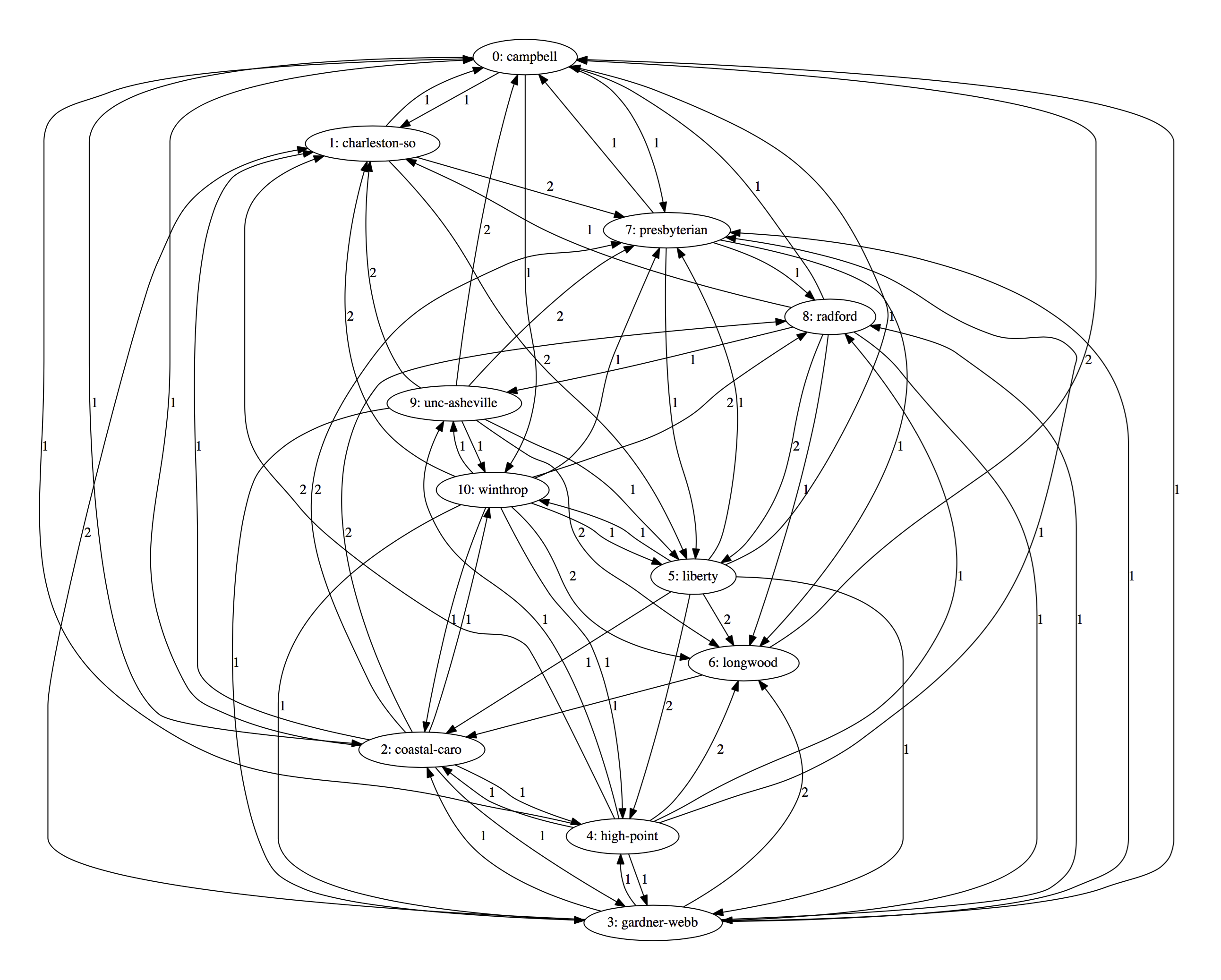
The numbers are not rankings. They simply indicate where the team is in the following alphabetical list of all the teams.
big_south = [
    'campbell','charleston-so','coastal-caro','gardner-webb','high-point',
    'liberty','longwood','presbyterian','radford','unc-asheville','winthrop'
]
More importantly, the numbers indicate how the teams correspond to the rows and columns of the following adjacency matrix.
import numpy as np
M = np.matrix([
    [0, 1, 1, 0, 0, 0, 0, 1, 0, 0, 1],
    [1, 0, 0, 0, 0, 2, 0, 2, 0, 0, 0],
    [1, 1, 0, 1, 1, 0, 0, 2, 2, 0, 1],
    [1, 2, 1, 0, 1, 0, 2, 1, 1, 0, 0],
    [1, 2, 1, 1, 0, 0, 2, 1, 1, 1, 0],
    [1, 0, 1, 1, 2, 0, 2, 1, 0, 0, 1],
    [2, 0, 1, 0, 0, 0, 0, 0, 0, 0, 0],
    [1, 0, 0, 0, 0, 1, 1, 0, 1, 0, 0],
    [1, 1, 0, 1, 0, 2, 1, 0, 0, 1, 0],
    [2, 2, 0, 1, 0, 1, 2, 2, 0, 0, 1],
    [0, 2, 1, 1, 1, 1, 2, 1, 2, 1, 0]
])
Now, in this example, the number of games varies from team to team, thus let's normalize. Here are the number of games that each team has played to this point:
MpMT = M+M.transpose()
games_played = [row.sum() for row in MpMT]
games_played
We'll go through essentially the same process that we went through before, though we'll normalize the matrix by dividing each row by the number of games that the corresponding team played.
M2 = np.matrix([[M[i,j]/games_played[i] for j in range(len(M))] for i in range(len(M))])
vals, vecs = eig(M2)
max_idx = np.argsort(abs(vals))[-1]
vec = abs(vecs[:,0])
ranking = np.argsort(vec).tolist()
ranking.reverse()
ranking
Here are the teams listed in that order:
[big_south[i] for i in ranking]
And their relative strengths, according to the eigenvector.
[vec[i] for i in ranking]
The entire NCAA
As we move to much larger data sets, there are new issues to think about. Obviously, we don't want to just type in thousands of entries into a large matrix; we'll have to work programmatically. In addition, there are often more efficient data structures to work with. Suppose we want to rank the whole NCAA, for example. We'll need to read and manipulate data from a file. I've stored a JSON file containing all division I results on our webspace for exactly this purpose. You can access it like so:
import requests, json
from zipfile import ZipFile
from io import BytesIO

response = requests.get(
    "http://marksmath.org/classes/Spring2016NumericalAnalysis/ncaa_basketball_data.json.zip"
)
zf = ZipFile(BytesIO(response.content))
json_string = zf.read('ncaa_basketball_data.json').decode('utf-8')
ncaa_bball_data_json = json.loads(json_string)
Now, ncaa_bball_data_json is just a Python dictionary with two keys:
ncaa_bball_data_json.keys()
The meta_data stores a little information about the file.
ncaa_bball_data_json['meta_data']
The vast majority of the info is in the 'data' key, which is a list with 344 elements.
len(ncaa_bball_data_json['data'])
Each element is a dictionary that looks like so:
ncaa_bball_data_json['data'][303]
Note that all the game results for this team are stored in 'games'.
Now, we can use this to build a much larger matrix to generate rankings for the entire NCAA. This is where we need to think about the appropriate data structure to deal with a larger data set. Our adjacency matrix is an example of a sparse matrix, i.e. the vast majority of its entries are zero. This is simply because most teams don't actually play one another. In fact, to the date that this file was generated there have been fewer than $9,000$ games played. We can get the exact count as follows:
data = ncaa_bball_data_json['data']
n = len(data)
sum([len(data[i]['games']) for i in range(n)])
This might seem like a lot but there are well over $100000$ potential matchups.
n*(n-1)
Thus, well over 90% of our entries are zeros and using a sparse representation should be a significant savings in terms of memory. More than that, if we multiply two sparse matrices, we don't need to even try most mulitplications. Thus, there are algorithms for matrices that typically run much faster, assuming the matrix is actually sparse. To compute eigenvalues, for example, we'll use scipy.sparse.linalg.eigs. Even better, eigs allows us to compute just the dominant eigenvalue/eigenvector pair, which is exactly what we need.
OK, let's actually do it. In the code that follows the entries $m_{ij}$ of the sparse matrix $M$ take the score of the game into account, as well as who actually won the game. In principle, this should give us a somewhat better ranking.
from scipy.sparse.linalg import eigs
from scipy.sparse import dok_matrix
import numpy as np
data = ncaa_bball_data_json['data']
teams = [team['name'] for team in data]
n = len(teams)
M = dok_matrix((n,n))
for i in range(n):
    games = data[i]['games']
    number_of_games = len(games)
    for game in games:
        opponent = game['opponent']
        if opponent in teams:
            j = teams.index(opponent)
            score = game['score']
            winning_score = max(score)
            losing_score = min(score)
            win_or_loss = game['result']
            if win_or_loss == "W":
                bonus = 1
                numerator = winning_score
            elif win_or_loss == "L":
                bonus = 0
                numerator = losing_score
            M[i,j] = M[i,j] + (bonus+numerator/(winning_score+losing_score))/number_of_games
And here is the top 10:
value, vector = eigs(M, which = 'LM', k=1)
vector = abs(np.ndarray.flatten(vector.real))
order = list(vector.argsort())
order.reverse()
ranking = [teams[i] for i in order]
ranking[:10]
Here's where UNCA fits in:
ranking.index('unc-asheville')