Sampling distributions and confidence intervals
Recently, we've discussed discrete random variables and their distributions. Today, we'll take a look at the process of sampling as a random variable itself. From this perspective, there's a distribution associated with sampling and an understanding of this distribution allows us to estimate how close statistics computed from the sample are to the corresponding parameters for the whole population. Thus, we're laying the foundation for inference - the process of drawing quantitative conclusions from our data.
This is very much like sections 5.1 and 5.2 of our text, though with an emphasis on means of numerical data rather than proportions in categorical data.
Sampling as a random variable
The process of computing a statistic based on a random sample can be thought of a random variable in the following sense: Suppose we draw a sample of the population and compute some statistic. If we repeat that process several times, we'll surely get different results.
Since sampling produces a random variable, that random variable has some distribution; we call that distribution the sampling distribution.
Example
Suppose we'd like to estimate the average height of individuals in a population. We could do so by selecting a random sample of 100 folks and finding their average height. Probably, this is pretty close to the actual average height for the whole population. If we do this again, though, we'll surely get a different value.
Thus, the process of sampling is itself a random variable.
Example (cont)
Let's illustrate this with Python. Recall that we've got a data set with the heights (and more) of 20000 individuals. Let's select 10 random samples of size 100 from that data set and compute the average height for each. Here's how:
import pandas as pd
df = pd.read_csv('https://www.marksmath.org/data/cdc.csv')
[df.height.sample(100).mean() for i in range(10)]
Looks like the actual average height of the 20000 folks in our CDC data set might be 66 or 67 point something. In fact, we can compute this exactly, since 20000 is not so huge for our computer, but in the general situation (like dealing with the whole US population), this can't be done.
The key questions in statistical inference
- What does the statistic (the computation from the sample) tell us about the parameter (the value for the whole corresponding population)?
More precisely:- How close can we expect the statistic to be to the parameter?
- How confident can we be in any assertions we make about the parameter?
Standard error
Since sampling is a random variable with a distribution that, distribution has a standard deviation. We call that standard deviation the standard error. Generally, the standard error depends on two things:
- The standard deviation $\sigma$ of the corresponding population parameter and
- The sample size $n$.
Standard error for a sample mean
For a sample mean, the standard error is $$\sigma/\sqrt{n},$$ which decreases with sample size.
We can understand where the $\sigma/\sqrt{n}$ comes from using the additivity of means and variances. Suppose that $X$ represents the random height of one individual. If we grab $n$ individuals, we might represent their heights as $$X_1,X_2,\ldots,X_n$$ and their average height as $$\bar{x} = \frac{X_1 + X_2 + \cdots + X_n}{n}.$$ Of course, we know that the standard deviation of the numerator is $\sqrt{n}\sigma$, thus the standard deviation of $\bar{x}$ is $$\frac{\sqrt{n}\,\sigma}{n} = \frac{\sigma}{\sqrt{n}}.$$
A computer experiment
We can illustrate standard error by running a little computer experiment. Suppose we have a large dataset of 20000 values. We grab a small sample of size 1, 4, 16, 32, or 64 from that dataset. We then compute the average of the sample. As it turns out, the spread of each histogram seems to be about half as much as the previous.
Confidence intervals
The computation of a sample mean is not exact; it has variability. Thus, rather than asserting that population mean is some specific value based on the sample mean, we often claim that the population mean probably lies in some interval and we do so with some level of confidence.
Forumula
The confidence interval for a sample mean $\bar{x}$ has the form $$[\bar{x}-ME, \bar{x}+ME],$$ where $$ME = z^* \times SE$$ is called the margin of error.
Let's pick this apart a bit. Recall that the standard error $SE$ is just another name for the standard deviation of the sample mean. The number $z^*$ is then multiplier that indicates how many standard deviations away from the mean we'll allow our interval to go. A common choice for $z^*$ is 2, which implies a $95\%$ level of confidence in our interval since we know that $95\%$ of the population lies within 2 standard deviations from the mean.
A computer example
Returning to our CDC data set of 20000 individuals that includes their heights, let's draw a random sample of 100 of them and write down a $95\%$ confidence interval for the average height of the population. We begin by getting the data, drawing the sample, and computing the mean of the sample.
heights = df.height.sample(100)
xbar = heights.mean()
xbar
Computer example (cont)
Now, our confidence interval will have the form $$[\bar{x} - ME, \bar{x} + ME].$$ We just need to know what $ME=z^*\times SE$ is. We first compute $SE=\sigma/\sqrt{n}$ where we take $\sigma$ to be the standard deviation of the sample, which we can compute directly:
from numpy import sqrt
s = heights.std()
se = s/sqrt(100)
se
Computer example (cont)
Now, for a $95\%$ level of confidence, we take $z^*=2$. Thus our margin of error is
me = 2*se
me
And here's our confidence interval:
[xbar - me, xbar + me]
Thus, we have a $95\%$ level of confidence that the actual mean lies in that interval.
Computer example (finalized)
In this particular example, since the population size of 20000 is not too large and already resides in computer memory, we can compute the actual population mean:
df.height.mean()
We should emphasize though, that we cannot typically do this!
A homework type example
Suppose we draw a random sample of 36 beagles and find their average weight to be 22 pounds with a standard deviation of 8 pounds. Use this information to write down a $95\%$ confidence interval for the average weight of beagles.
Solution: Our answer should look like
$$[\bar{x} - ME, \bar{x} + ME] = [22-z^*\times SE,22+z^*\times SE].$$Now
$$SE = \sigma/\sqrt{n} = 8/6 \approx 1.33$$and our rules of thumb tell us to take $z^* = 2$ for a $95\%$ level of confidence. Thus, our confidence interval is
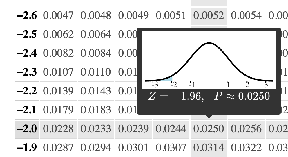
$$[22 - 2\times1.33, 22+2\times1.33] = [19.34,24.66].$$As we'll see in our table though, a better answer might use $z^*=1.96$.
Varying the confidence level
What if we're not looking for a $95\%$ level of confidence? Rather, we might need quite specifically a $98\%$ confidence interval or a $99.99\%$ confidence interval. We simply find the $z^*$ value such that the area under the standard normal shown below is our desired confidence level.

Varying confidence level (cont)
If, on the other hand, we needed a $98\%$ level of confidence, we'd need to look at this row:
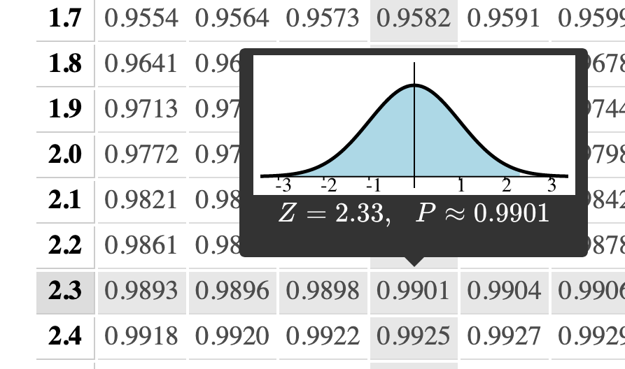
Thus, it looks like $z^* = 2.33$ should do.
Beagles again
In the beagle example, our 98% confidence interval would be
$$[22 - 2.33\times1.33, 22+2.33\times1.33] = [18.9,25.1].$$Note that the interval needs to be bigger to be more confident.
Conditions to check
Finally, we should mention that in order for this technique to work, the sample means must be normally distributed. This does not require that the underlying data is normally distributed For example, weight is not typically normally distributed but the sample means of weight are. Here are the conditions that we need to check to make sure these ideas are applicable:
- A simple random sample
- Independence
- Large enough (typically, at least 30) but
- Need less than 10% of population for independence