More on the Normal
Today, we're going to review a bit about the normal distribution and push it further so that we can assess all kinds of probabilities associated with it.
This is all from section 4.1.
Formulae
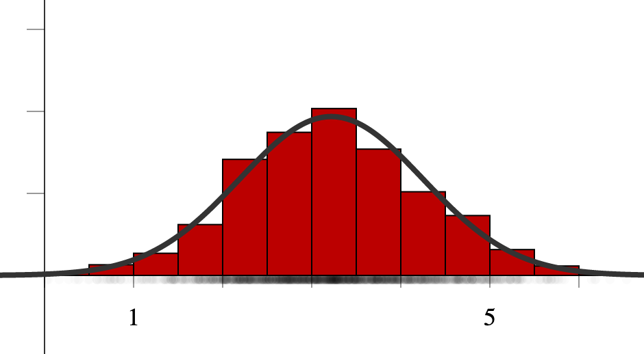
More specifically, the curve on the previous slide is the normal curve whose mean and standard deviation is the same as the data.
If the raw data is numerical in nature, say ${x_1,x_2,\ldots,x_n}$, then we use software to compute
$$\mu \approx \bar{x} = \frac{x_1+x_2+\cdots+x_n}{n}, \text{ and }$$$$\sigma^2 \approx s^2 = \frac{(x_1-\bar{x})^2 + (x_2-\bar{x})^2 + \cdots + (x_n-\bar{x})^2}{n-1}.$$If the data can be broken up into two categories, say success of an experiment with probability $p$ vs failure with probability $1-p$ resulting from $n$ trials, then
$$\mu \approx np \: \text{ and } \: \sigma \approx \sqrt{np(1-p)}.$$Models
A key point about the normal distribution is that we can use it to model our data. We might run more trials of our experiment or draw a different random sample of folks to survey and get slightly different data. If we have similar sample sizes and conditions, though, the same normal distribution should work.
We can also explore completely different questions and, again - as long as we can expect the daa to be normally distibution with understood mean and standard devation, we can analyze that data with the normal model.
Furthermore, the central limit theorem is always lurking in the background ensuring that data obtained via an aggregation or averaging process of independent observations will be normally distributed.
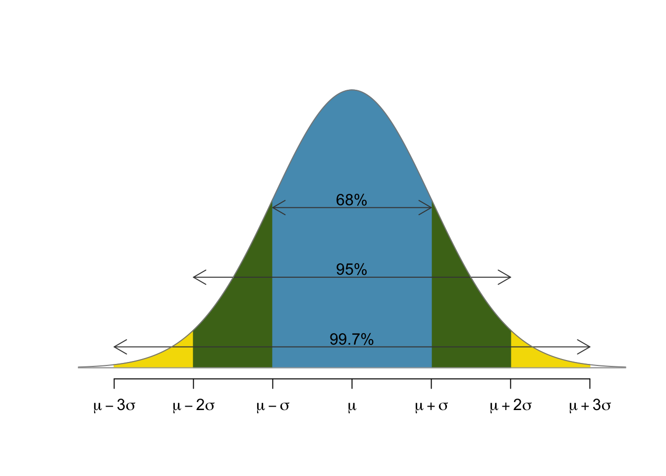
Quantified picture
To understand the model, you'll always want to keep this picture in mind. The percentages give us a rough understanding of the distribution.
Example
Scores on the SAT exam are, by design, normally distributed with mean 500 and standard deviation 100.
Using that fact, at what percentile is a score or 700?
Why normal?
In fact, SAT scores must be approximately normally distributed simply because they result by summing the scores obtained from a fairly large battery of mostly independent questions. Thus, the central limit theorem guarantees normality; to set the mean to 500 and standard deviation to 100 is then simply a matter of rescaling.
Example (cont)
First, let's make sure we understand the question: Assuming we score a 700 on the SAT, then what percentage of folks can we expect scored below our score?
Solution
The first observation is that $$700 = 500 + 2\times100 = \mu+2\sigma.$$ That is, 700 is two standard deviations past the mean.
Now, our rules of thumb tell us that $95\%$ of the population lies within two standard deviations of the mean and only $5\%$ outside of that. Of that $5\%$, only half (or $2.5\%$) scored higher than us and the other $2.5\%$ scored far lower.
Thus, our 700 puts us at the $97.5^{\text{th}}$ percentile.
The Z-Score
Here's another way to think about it that will useful as we move to trickier examples. Recall that, if $X$ is normally distributed with mean $\mu$ and standard deviation $\sigma$, then we can translate $X$ to a standard normal via
$$ Z = \frac{X-\mu}{\sigma}. $$Computing this for a specific value of $X$ results in the $Z$-score for that value.
For the SAT example, the $Z$-score of 700 given $\mu=500$ and $\sigma=100$ is
$$ Z = \frac{700-500}{100} = 2. $$Furthermore, the area under the standard normal to the left of 2 is about $0.975$.
The picture
The picture below illustrates the standard normal and the SAT normal for this problem.

If you're thinking those are the same picture with different numbers, then you're exactly right - that's the point!
More precise computations
What if you score a 730 or a 420 on the SAT? Or what if you're 65.5 inches tall and you'd like to know how that compares to others in our CDC data set?
Then, you'll need to perform more precise area computations for regions under the normal distribution.
There's generally two ways to accomplish this:
- Using a standard table
- Using software
A portion of a table
Here's a little portion of a table to help convey the idea. There are dynamic HTML and static webpage versions on our class webpage.
Standard examples
Suppose that $Z$ is a random variable that has a standard, normal distribution. Then find
- $P(0<Z<1)$
- $P(-1<Z<1)$
- $P(Z<1)$
- $P(0<Z<1.5)$
- $P(Z>1.5)$
- $P(-1.23 < Z < 2.31)$
- The value $z_0$ of $Z$ for which $$P(0 < Z < z_0)=0.25.$$
Normal examples
Suppose that $X$ is a normally distributed random variable with mean $\mu=17.5$ and standard devation $\sigma=4.2$. Then find
- $P(17.5<X<25)$
- $P(10<X<25)$
- $P(X<25)$
- $P(12.3<X<22.1)$
Height
Let's return to a data based example. The following code reads our CDC data and computes the mean and standard deviation for the height of the women in that study. It then computes proportion of women under 65.5 inches tall.
import pandas as pd
from scipy.stats import norm
df  = pd.read_csv('https://marksmath.org/data/cdc.csv')
df = df[df.gender=='f']
m = df.height.mean()
s = df.height.std()
p = norm.cdf(65.5,m,s)
[m,s,p]
Let's make sure we can compute this with a table as well. Of course, we'll need a Z-score to do so:
(65.5-m)/s