Continuous random variables
Last time we learned that a random variable $X$ is a random process with some numerical outcome and we focused on discrete random variables - i.e. random variables that generate integer values. Today, we'll continue our discussion of random variables but focus on continuous random variables that can, in principle, generate any real number. We'll also meet the normal distribution and explore its relationship with the binomial distribution.
This material is mostly discussed in sections 3.4, 3.5, and 4.1. There material describing the relationship between the binomial and normal distributions is discussed in section 4.3.
Examples
Even last time, we met a few continuously distributed random variables:
- Example A: Let $X$ be the average number of points that Ohio State beats Michigan by until Michigan (someday, a long time from now) finally wins,
- Example B: Find somebody and choose $X$ to be a very precise measure of their height,
- Example C: Randomly choose a college and choose $X$ to be the average salary of all the professors.
The tricky thing is trying to figure out how to describe the distribution of a continuously distributed random variable.
The uniform distribution
The continuous, uniform distribution is probably the simplest example of a continuous distribution in general. Suppose I pick a real number between $-1$ and $1$ completely (and uniformly) at random. What does that even mean?
I suppose that the probability that the number lies in the left half of the interval (i.e. to the left of zero) should be equal to the probability that the number lies in the right half. Phrased in terms of a probability function applied to events, we might write
$$P(X<0) = P(X>0) = \frac{1}{2}.$$The uniform distribution (cont)
Pushing the previous slide a bit further, suppose we a number uniformly at random from an interval $I$. The probability of picking a number from a sub-interval should be proportional to the length of that sub-interval.
If the big interval $I$ has length $L$ and the sub-interval $J$ has length $\ell$, then I guess we should have
$$P(X \text{ is in } J) = \ell/L.$$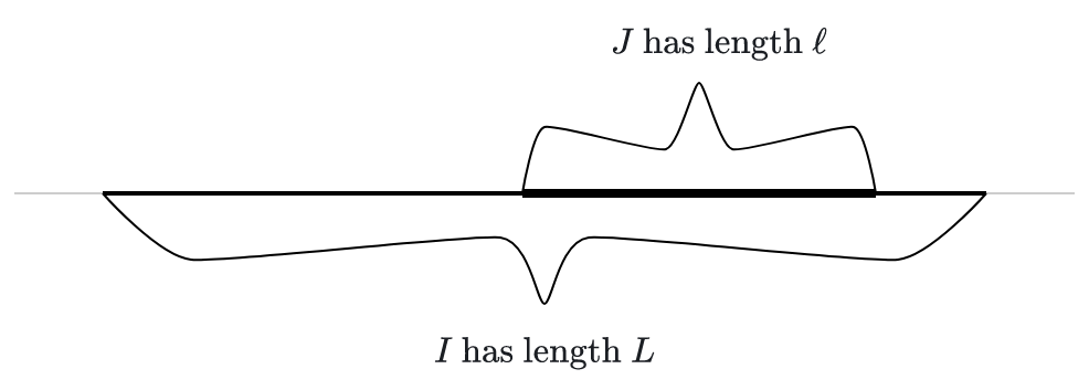
Example
Suppose we pick a number $X$ uniformly at random from the interval $[-10,10]$. What is the probability that the number lies in the interval $[1,3]$?
Solution: We simply divide the length of the sub-interval by the length of the larger interval to get
$$P(1<X<3) = \frac{2}{20} = 0.1.$$Note that we've indicated the event using the inequality $1<X<3$, as we will typically do.
Visualizing the continous uniform distribution
A common way to visualize continuous distributions is to draw the graph of a curve in the top half of the $xy$-plane. The probability that a random value $X$ with that distribution lies in an interval is then the area under the curve and over that interval. This curve is often called the density function of the distribution.
In the case of the uniform distribution over an interval $I$, the "curve" is just a horizontal line segment over the interval $I$ at the height 1 over the length of $I$. In the picture below, for example, $I=[0,2]$. On the left, we see just the density function for the uniform distribution over $I$. On the right, we see the area under that density function and over the interval $[0.5,1]$. The area is $1/4$ since $$P(0.5<X<1) = 1/4.$$

The normal distribution
That brings us to the normal distribution - the most important distribution in elementary statistics!
Suppose we go outside, grab the first person we see and measure their height. Accoring the data in our CDC data set, the average person has a height of about 67.18 inches. I suppose that our randomly grabbed person will have a height of close to that 67.18 inches. In fact, most people have a height of $$67.18 \pm 4 \text{ inches}.$$ Of course, there are people taller than 72 inches and shorter than 62 inches, but the number of folks you find of a certain height grows more sparse as we move away from the mean.
A normal density function
If we try to plot a curve that meets the criteria of a density function for heights, I guess it might look something like so:

Note that the area is concentrated near the mean of $67.18$. The shaded area represents 1 standard deviation (or $4.12$) away from the mean; which represents about $68\%$ of the population. There are people 2 and even 3 standard deviations away from the mean but they taper off rapidly.
The family of normal distributions
There's more than one normal distribution; there's a whole family of them - each specified by a mean and standard deviation.
All normal distributions have the same basic bell shape and the area under every normal distribution is one.
The mean $\mu$ of a normal distribution tells you where its maximum is.
The standard deviation $\sigma$ of a normal distribution tells you how concentrated it is about its mean.
The standard normal distribution is the specific normal with mean $\mu=0$ and standard deviation $\sigma=1$.
The family album
The interactive graphic below shows how the mean and standard deviation determine the corresponding normal distribution.
Standardizing normals
Any normally distributed random variable $X$ (with mean $\mu$ and standard deviation $\sigma$) can be translated to the standard normal $Z$ via the formula
$$ Z = \frac{X-\mu}{\sigma}. $$Given a normally distributed random variable $X$ that obtains the value $x$, the computation
$$ z = \frac{x-\mu}{\sigma} $$is called the $Z$-score for $x$.
The behavior of the standard normal
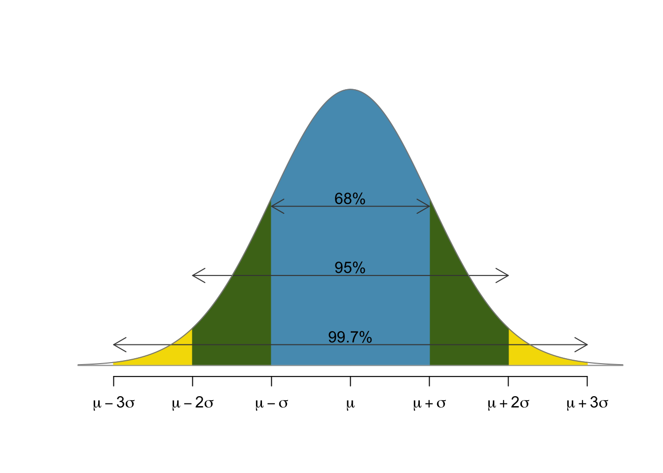
Since we can relate any normally distributed random variable to the standard normal, it's of great interest to fully understand the standard normal. There is a statistical rule of thumb for this purpose called the 68-95-99.7 rule that states that
- 68% of the population lies within 1 standard deviation of the mean,
- 95% of the population lies within 2 standard deviations of the mean, and
- 99.7% of the population lies within 3 standard deviations of the mean.
A picture of the standard behavior
Example
Let's suppose that the mean life expectancy of a cat is 14 years with a standard deviation of 2.5 years. Assuming that the cats' life spans are normally distributed, is it reasonable to expect a cat to live to 22 years old?
Solution: Well, the $z$-score for a 22 year old kitty cat would be $$Z = \frac{22-14}{2.5} = 3.2.$$ As we know, only $0.3\%$ of cats live beyond a $z$-score of 3, so a 22 year old cat would be quite rare indeed.
Binomials and Normals
The interactive tool below allows you to play with the parameters defining a binomial distribution and shows how the correspsonding normal fits in.
The central limit theorem
The central limit theorem is the theoretical explanation of why the normal distribution appears as the limit of binomials above and, therfore, so often in practice. Suppose that $X$ is a random variable which we evaluate a bunch of times to produce a sequence of numbers: $$X_1, X_2, \ldots, X_n.$$ We then compute the average of those values to produce a new value $\bar{X}$ defined by $$\bar{X} = \frac{X_1 + X_2 + \cdots + X_n}{n}.$$ The central limit theorem asserts that the random variable $\bar{X}$ is normally distributed. Furthermore, if $X$ has mean $\mu$ and standard deviation $\sigma$, then the mean and standard deviation of $\bar X$ are $\mu$ and $\sigma/\sqrt{n}$.
Note that all of this is true regardless of the distribution of $X$!