Discrete Random Variables
and their distributions
Last week, after finishing up our discussion of data, we jumped into probability theory. This week, we're going to push our knowledge of probability theory further to talk about random variables. Today's material is covered in sections 3.4 and 4.3 of our textbook. (Yes, it jumps around a bit.)
As we go through this, we'll have occasion to review some of our material on probability as well.
Ultimately, everything we do is in an effort to understand data. While some of this material may seem a bit abstract, in reality these are the very tools that we use to model data. Thus, to understand the model is to understand data itself.
Random variables
On page 116, the concept of a random variable $X$ is defined to be a random process with some numerical outcome.
- Example 0: Choose $X$ to be the sum of the scores of the next Ohio State - Michigan game
- Example 1: Flip a coin and write down
- $X=1$ if the coin lands heads or
- $X=0$ if the coin lands tails
- Example 2: Roll a standard six sided die and write down the number that comes up.
- Example 3: Roll a 10 sided die and write down
- $X=1$ if the roll comes up 1, 2, or 3,
- $X=2$ if the roll comes up 4, 5, 6, or 7, or
- $X=3$ if the roll comes up 8, 9, or 10
All these examples produce only integer values and are called discrete random variables. In the language of probability theory that we developed last week, we would say that the sample space is the set of integers
Continuous random variables
There are certainly random variables that can, in principle, produce any real number.
- Example A: Let $X$ be the average number of points that Ohio State beats Michigan by until Michigan (someday, a long time from now) finally wins,
- Example B: Find somebody and choose $X$ to be a very precise measure of their height,
- Example C: Randomly choose a college and choose $X$ to be the average salary of all the professors.
These are all continuous random variables. In the language of probability theory that we developed last week, we would say that the sample space is the set of real numbers.
Continuous distributions are certainly very important and we will dive into them in more detail next time. Today, though, we will focus on discrete distributions.
Distributions for discrete random variables
Roughly, the distribution of a random variable tells you how likely that random variable is to produce certain outputs. For a discrete random variable, this boils down to listing out the probability that the random variable hits every specific value.
On page 87 of our text, the distribution of a discrete random variable is defined to be a table of all the possible outcomes together with their probabilities.
For example 3 above, we might write
| X | 1 | 2 | 3 |
|---|---|---|---|
| p | 3/10 | 4/10 | 3/10 |
Note the all the probabilities should be non-negative and they should sum to one.
Functional notation
An alternative is to specify the values of a function $P$ for the possible values of $X$. For example, the previous table could be written:
- $P(X=1) = 3/10$
- $P(X=2) = 4/10$
- $P(X=3) = 3/10$
As we'll see next time, this notation will extend in a natural way to continuous distributions.
Pictorial representation
A final alternative is to represent a discrete distribution with a plot.

A large discrete distribution
Pictorial representations of discrete distributions make particular sense when there are a large number of possibilities. The image below portrays a discrete distribution where the sample space is the set of integers between 1 and 100 and smaller numbers are more likely to be chosen than larger numbers.

The discrete, uniform distribution
If the sample space of a discrete distribution consists of $n$ consecutive integers, each of which has probability $1/n$, then the distribution is said to be uniform. For example, we might write: $$ P(X=i) = \begin{cases} 0.01 & \text{if } 1 \leq i \leq 100 \\ 0 & \mbox{otherwise.} \end{cases} $$ This can be visualized like so:

The roll of a six-sided die or the flip of a coin can each be represented with a discrete uniform distribution.
Rolling Two D6
Suppose we roll 2 six-sided die. We then form a random variable $X$ by adding the totals on the two die. We could get any number between 2 (snake eyes) and 12 (box cars) - but they are not all equally likely. According to the table on page 87 of our text, the probabilities are:
| 2 | 3 | 4 | 5 | 6 | 7 | 8 | 9 | 10 | 11 | 12 |
|---|---|---|---|---|---|---|---|---|---|---|
| 1/36 | 2/36 | 3/36 | 4/36 | 5/36 | 6/36 | 5/36 | 4/36 | 3/36 | 2/36 | 1/36 |
To understand this, note that, when we roll two die they are independent of one another. Thus the probability of getting any particular pair is $$\frac{1}{6}\times\frac{1}{6} = \frac{1}{36}.$$ Thus, the probability of getting any specific sum is the number of ways to get that sum times $/36$.
Rolling Two D6 - Illustrated
Here's an illustration of the idea of the number of ways to get certain sums of die rolls.
The binomial distribution
The binomial distribution is a discrete distribution that plays a special role in statistics for many reasons. Importantly for us, the binomial distribution allows us to see how a bell curve (in fact the normal curve) arises as a limit of other types of distributions.
Flipping a coin five times
Suppose we flip a coin 5 times and count how many heads we get. This will generate a random number $X$ between 0 and 5 but they are not all equally likely. The probabilities are:
- $P(X=0)=1/32$
- $P(X=1)=5/32$
- $P(X=2)=10/32$
- $P(X=3)=10/32$
- $P(X=4)=5/32$
- $P(X=5)=1/32$
Note that the probability of getting any particular sequence of 5 heads and tails is $$\frac{1}{2^5} = \frac{1}{32}.$$ That explains the denominator of 32 in the list of probabilities.
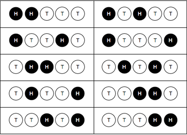
Flipping a coin five times (cont)
The numerator in the table on the previous slide is the number of ways to get the sum. For example, there are 10 ways to get 2 heads in 5 flips:
Interactive binomials
The interactive tool below allows you to play with the parameters defining a binomial distribution.
Mean and standard deviation
The mean and standard deviation that we learned for data can be extended to random variables using the idea of a weighted average.
Mean or expectation
The expectation of a discrete random variable is $$ E(X) = \sum x_i P(X=x_i) = \sum x_i p_i.$$ We might think of this as a weighted mean.
Examples
Weighted die roll
Recall our weighted die roll with probability distribution
| X | 1 | 2 | 3 |
|---|---|---|---|
| p | 3/10 | 4/10 | 3/10 |
The expected value of a roll of this die is $$1\frac{3}{10} + 2\frac{4}{10} + 3\frac{3}{10} = 2.$$
Weighted coin flip
I've got a weighted coin that comes up heads $75\%$ of the time, in which case I write down a one. If it comes up tails, I write down a zero. The expectation associated with one flip is $$E(X) = 1\times \frac{3}{4} + 0 \times \frac{1}{4} = \frac{3}{4}.$$
Standard deviation
The variance of a discrete random variable $X$ is $$\sigma^2(X) = \sum (x_i - \mu)^2 p_i.$$ We might think of this as a weighted average of the squared difference of the possible values from the mean. The standard deviation is the square root of the variance.
Examples
Weighted die roll
The variance of our weighted die roll in example above is $$(1-2)^2\frac{3}{10} + (2-2)^2\frac{4}{10} + (3-2)^2\frac{3}{10} = \frac{6}{10}.$$
Weighted coin flip
The variance of our weighted coin flip is $$\sigma^2(X) = (1-3/4)^2\frac{3}{4} + (0-3/4)^2 \frac{1}{4}=\frac{3}{16}.$$
Combining distributions
One nice thing about expectation and variance is that they are additive. That is, if $X_1$ and $X_2$ are both random variables, then $$E(X_1 + X_2) = E(X_1) + E(X_2)$$ and $$\sigma^2(X_1 + X_2) = \sigma^2(X_1) + \sigma^2(X_2).$$
Example
Suppose I flip my weighted coin that comes up heads 75\% of the time 100 times and let $X_i$ denote the value of my $i^{\text{th}}$ flip. Thus, $$X_1 + X_2 + \cdots X_{100}$$ represents the total number of heads that I get and, by the additivity of expectation, we get $$E(X_1 + X_2 + \cdots X_{100}) = 100 \times \frac{3}{4} = 75.$$
Example (cont)
Similarly, for the variance we get $$\sigma^2(X_1 + X_2 + \cdots X_{100}) = 100 \times \frac{3}{16} = \frac{75}{4}.$$ Of course, this means that the standard deviation is $\sqrt{75/4}$.
Note: The standard deviation of one flip is $\sqrt{3/16} \approx 0.433013$ and the standard deviation of 100 flips is $\sqrt{75/4} \approx 4.33013$. The second is 10 times larger in magnitude but, relative to the total number of flips it's $0.0433013$, which is tens times smaller.
Mean and variance for binomial random variables
Suppose that $X$ is a random variable with
$$P(X=1)=p \text{ and } P(X=0)=1-p.$$Then, $$E(X) = p\times1+(1-p)\times0 = p$$ and $$\sigma^2(X) = p(1-p)^2 + (1-p)(0-p)^2 = p(1-p).$$ The standard deviation is then $$\sigma(X) = \sqrt{p(1-p)}.$$ These are forumulae that we will definitley use!
Repeated experiments
Now suppose that $S$ represents the sum of $n$ independent runs of $X$. Then, since mean and variance are additive, we have
$$E(S) = np,$$$$\sigma^2(S) = np(1-p),$$and $$\sigma(S) = \sqrt{np(1-p)}.$$
Example
Judging from our class survey, around $12.5%$ of the population has green eyes. Suppose we now draw a random sample of 150 people. Assuming our estimate to be a good one,
- How many people from the sample do we expect to have green eyes?
- What is the standard deviation associated with that process?
Solution
We expect about $150\times0.125 = 18.75$ people to have green eyes.
The standard deviation would be $$ \sigma \approx \sqrt{150\times0.125\times(1-0.125)} \approx 4.05. $$