Differential Equations - an overview

That's

• differential
• equations.

Let's make sure we understand both terms.

Equations

We learn of equations in precalculus or even pre-precalculus. Some examples include

• $x+1=2$
• $ax^2+bx+c = 0$
• $x^2 + 1 = 0$
• $\cos(x) = x$

We can also have systems of equations:

• $x+y=4,$
• $x-y=2$

Key features

Some of the key features of equations include:

• Equals signs (that's where the equa part comes from),
• variables (symbols representing numbers),
• type (linear, polynomial, transcendental),
• order of a polynomial equation,
• solutions (which might or might not be easy to find, if they exist at all).

Algebraic techniques

Inspection

Some equations are simple enough to be solved by inspection or, more honestly, guessing.

For example, it doesn't take too much imagination to find that $x+1=2$ has the solution $x=1$.

Algebraic manipulation

Some equations are a bit more involved. For example $3 x^2 + 5 = 32$ has the solutions $x=\pm3$. This is pretty easy to check but you might need to bring the 5 over, divide by 3, and take square roots to find those solutions.

Other equations involve more advanced techniques, like $x^2-x-1=0$, which probably requires the quadratic formual.

Qualitative techniques

Qualitative techniques essentially boil down to thinking geometrically.

For example, if we plot the graph $f(x)=x^2+1$, we see that it lies completly above the $x$-axis. Thus, the equation $x^2+1=0$ has no solution.

Similarly, if we plot the graphs of $y=\cos(x)$ and $y=x$ together, we see they intersect at exactly one point. Thus, the equation $\cos(x)=x$ has a unique solution.

If we design our plots carefully enough, we can get a reasonable estimate to the value of the solution. The picture below, which I made pretty easily with Python, indicates that the solution of $\cos(x)=x$ is around $3/4$.

import matplotlib.pyplot as plt
import numpy as np
x = np.linspace(-0.2,1.2,100)
y = np.cos(x)
plt.plot(x,y)
plt.plot([-0.2,1.2],[-0.2,1.2]);

Numeric techniques

Sometimes, qualitative techniques indicate the existence of a solution that we can't find algebraically. Often, though, we can use numeric techniques to find a decimal approximation to the solution.

One common technique for finding numerical solutions is called iteration: Given a real valued function $f$ and an initial value $x_0$, we recursively define $x_{i+1}=f(x_i)$. Under suitable hypotheses, this process will often converged to a fixed point of the function - i.e. a solution of $f(x)=x$.

For example, here's how to iterate $f(x)=\cos(x)$ from $x_0=3/4$ using Python:

import numpy as np
x = 3/4
for i in range(8):
    x = np.cos(x)
    print(x)

0.7316888688738209
0.7440470847887636
0.735733618187236
0.741338598887922
0.7375652963392665
0.7401080596152838
0.7383956911259042
0.7395493740083101

Cobweb plots

The process of iteratation can be visualized using a so-called cobweb plot. Here's the cobweb plot for the cosine:

$x_0$

$n$

Differential Equations

First off, differential equations are equations. Thus, they involve equalities of expressions involving unknowns; solutions of the equations are values of the unknowns that make the equations true.

The key difference and novel aspect is that the unknows represent functions rather than numbers. In addition, the equations involve derivatives of the unknown functions, as well as the function itself.

Examples

• $y'(x) = r y(x)$
• $y'(x) = -2 \, x \, y(x)$
• $P'(t) = kP(t)(1-P(t))$
• $x''(t) = -\omega^2 x(t)$

Note that there are three types of symbols here - functions (like $y$, $P$, or even $x$), variables (like $x$ or $t$), and parameters (like $r$, $k$, or $\omega$).

Often, we'll supress the functional variable. Thus the first equation might be written $y'=ry$.

Solutions

As with ordinary equations, a solution is a value (in this case a function) with the property that the equation is true when the unknown is replaced with the solution.

Example 1

If $y' = -2xy$, then one solution is $y(x) = e^{-x^2}$, though there are others.

Example 2

Given $y'=y$, you can probably find at least one solution by inspection.

Just as with ordinary equations, we'll discuss algebraic, qualitative, and numeric ways to find solutions.

Terminology

The order of a differential equation is the highest order derivative that appears in the equation.

• $2y'y + 1 = y^2 \text{ is first order}$
• $y''' = -k y' \text{ is third order.}$

A system of differential equations consists of more than one equation with more than one unknowns.

The pair of equations

• $y''=-x$
• $x''=y$

forms a second order system of equations.

Ordinary vs partial

When the unknown functions are functions of a single variable, the equation is called an ordinary differential equation or ODE.

When the unknown functions are functions of several variables, the equation is called an partial differential equation or PDE.

This class, Math 394, is devoted to the study of ODEs. Spring semester's Math 395 is devoted to PDEs.

Autonomous equations

When an ODE or system of ODEs can be expressed without explicit reference to the independent variable of the unknown functions, then it is called autonomous. We very often use this language when the independent variable refers to time.

Examples

The equation $x' = x$ is autonomous.

The equation $x' = -2t x$ is non-autonomus.

Initial value problems

Most of the ODEs we will meet have inifinitely many solutions but have a unique solution when an initial value is specified. An ODE together with such a specification is called an initial value problem or IVP.

Example

Consider consider the autonomous, first-order ODE $x'=x$. This has the general solution $$x(t) = c e^t.$$

Now suppose that, in addition to the ODE, we require the function $x$ to satisfy the initial condition $x(0)=2$. Then, $$x(0) = c e^0 = c = 2.$$ Thus, $c=2$ so that $x(t) = 2e^t$ is the only solution to the IVP.

First order ODEs

Chapter 1 of our text is devoted to first order, ordinary differential equations. Thus, we've got an equation involving a single function $x$ of single variable $t$ and just the first derivative $x'$. Assuming we can solve the equation for $x'$, we might write that equation in the form $$x' = f(t,x).$$ This is called the general form for a first order ODE.

Alternatively, we might write $$y' = f(x,y).$$ You should understand that we've just changed the names of the function and independent variable and you should be comfortable making this type of change. The first form is convenient when we are thinking of a quantity that changes with respect to time. The second form will be convenient when we try to understand a particular qualitative approach to visualizing first order ODEs.

Growth/Decay Equations

Consider the very simple yet extremely important, first order, autonomous equation:

$$y' = r y.$$

Note that $y$ represents a function whose variable we will assume is time $t$ and that $r$ is a parameter. There is a very simple and important interpretation of this equation:

The rate of growth or decay of $y$ is proportional to $y$ itself.

Put another way - the more $y$ you got, the faster $y$ will change.

Growth/Decay

There are lots of quantities that obey this type of equation, at least over some time span:

• Population
• Money
• Radioactive material (where $r<0$)

A solution

It's quite easy to find the general solution to $y'=ry$:

$$y(t) = c e^{rt}.$$

You can verify this solution by simply computing $y'$ and checking that the result is $ry$.

Note that when $r>0$, the quantity $y$ increases but that when $r<0$, the quantity $y$ decreases.

Finding the solution

Given a first order equation $y'=f(t,y)$, we can sometimes find a solution using separation of variables. Let's illustrate using our simple equation:

$$\frac{dy}{dt} = r\,y,$$

where we've replaced $y'$ with $\frac{dy}{dt}$ (that's part of the trick).

We treat $\frac{dy}{dt}$ like a fraction and try to get all $y$s on one side and all $t$s on the other:

$$\frac{1}{y}dy = r\,dt.$$

Finding the solution (cont)

We then integrate both sides:

$$\int\frac{1}{y}dy = \int r\,dt$$

to get

$$\log(y) = r\,t + c_1.$$

and apply the exponential to both sides to get

$$y = e^{r\,t+c_1} = c\,e^{r\,t},$$

where $c=e^{c_1}$.

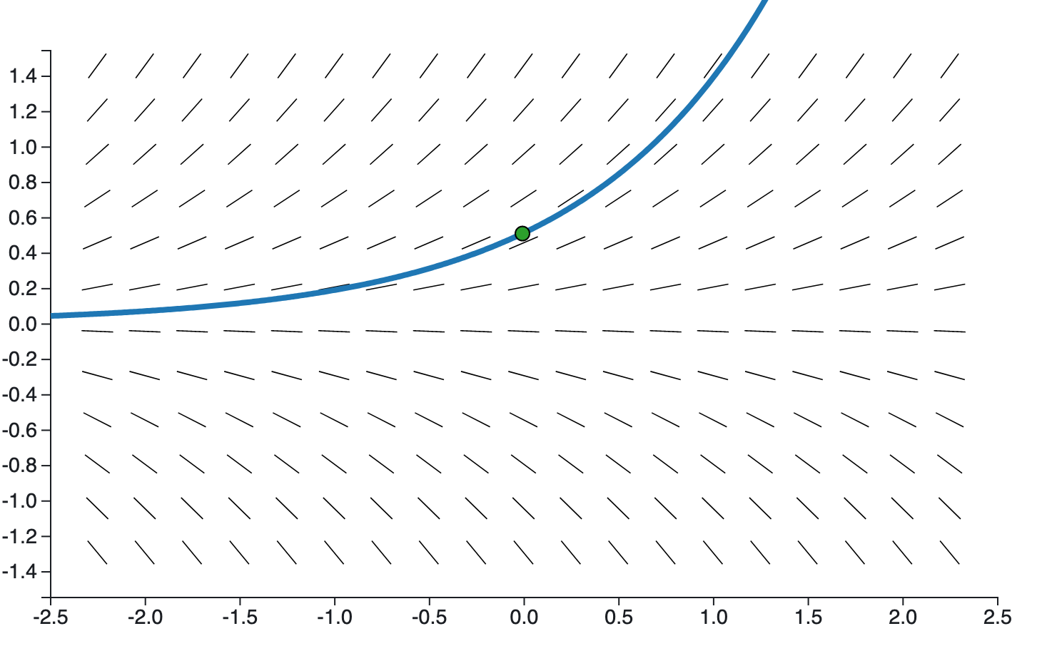
Visualizing the solution

Here's a view of the solution of $y'=y$ subject to $y(0)=1/2$ as it runs through its slope field.

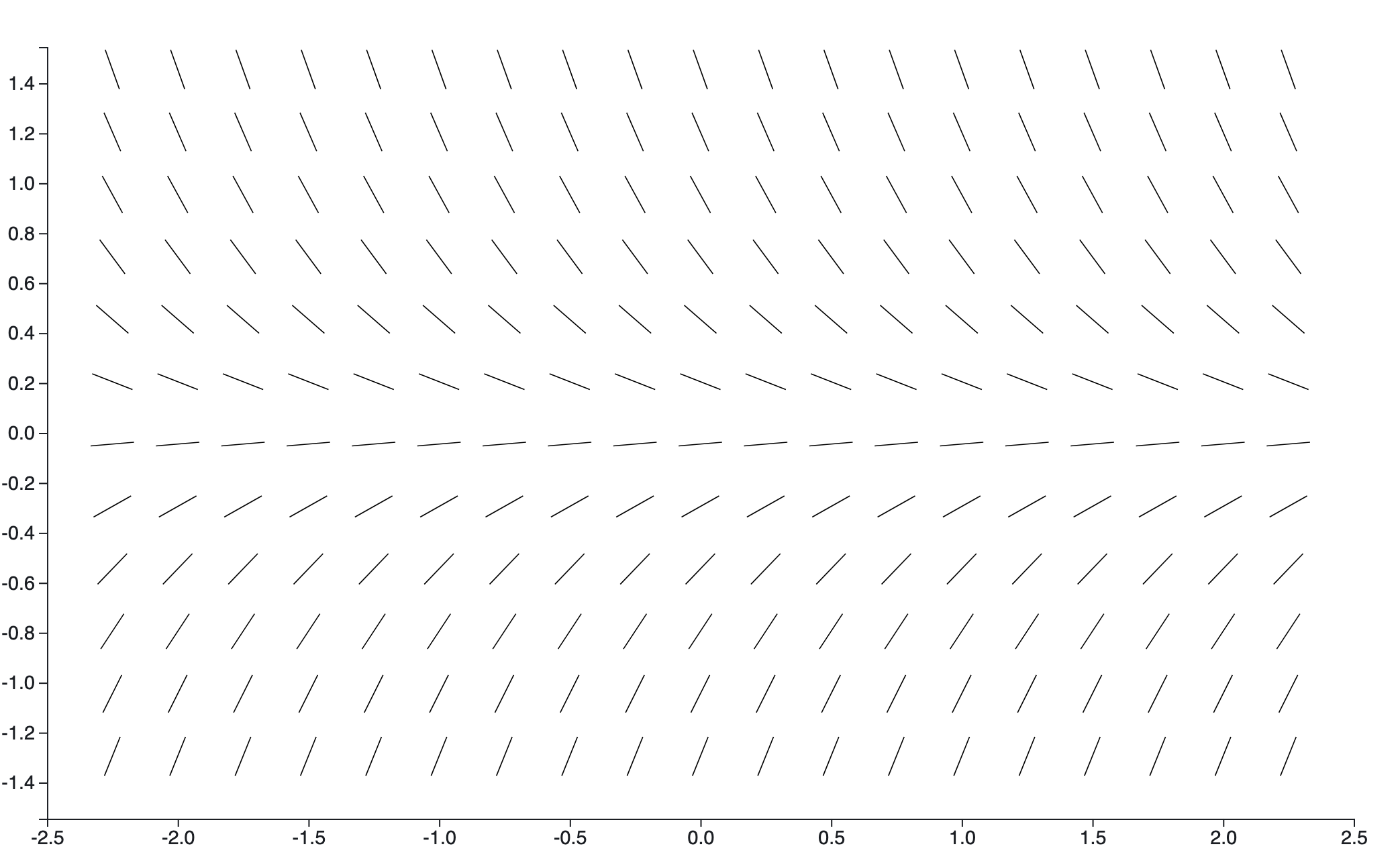
Slope fields

The slope field itself is a very important tool for qualitative analysis. We can draw one for any first order ODE written $y'=f(t,y)$.

At each point $(t,y)$ in a grid in the $ty$-plane, we draw a little line segment with slope $f(t,y)$.

Since $y' = f(t,y)$, this tells us the slope of any solution as it passes through any particular point.

To draw the graph of a solution, it's just matter of following the slope field!

Slope field example

Here's the slope field for $y' = -2y$.

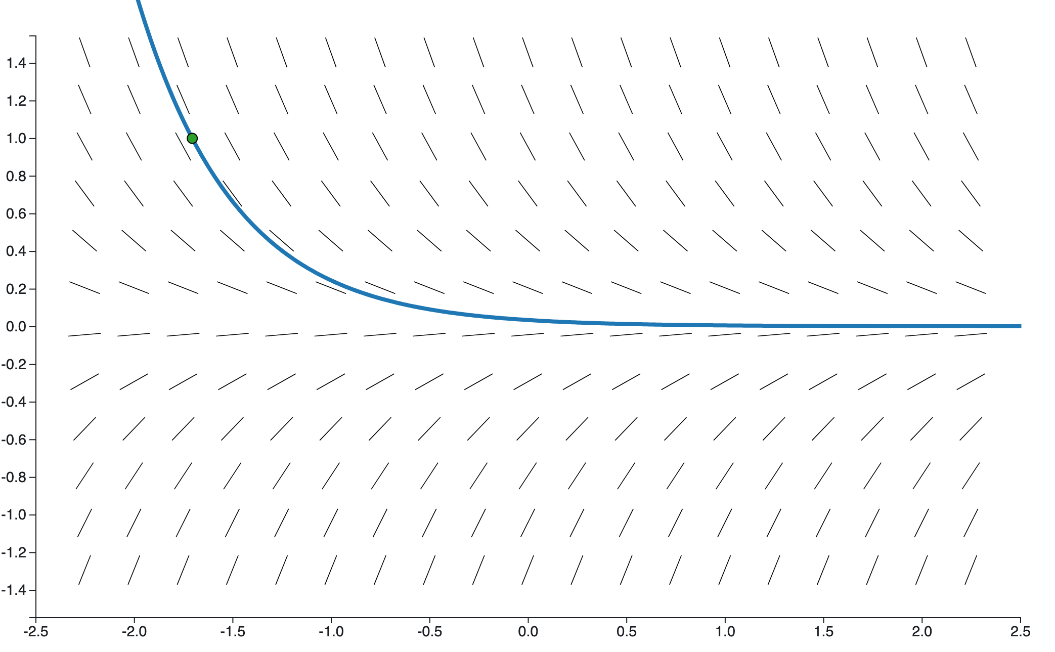
Slope field example (cont)

Here's the solution of $y' = -2y$ subject to $y(-1.5)=1$ as it passes through its slope field.