Numerically solve an IVP

mark · August 2020

(10 pts)

Produce and IVP of the form
$$
y' = r\,y\,\sin(y), : y(0)=1
$$
by choosing the decimals of $r$ to be the positions in the alphabet of your login name.
For example, my login name is mark and the positions of those letters are 13, 1, 18, and 11. Thus, for me, $r=0.1311811$ and my ODE is
$$
y' = 0.1311811 \, y \, \sin(y).
$$
Find the value of $t$ for which $y(t)=3$.

mark · August 2020

So, here's how I might approach it. First, my IVP is

$$
y' = 0.1311811 \, y \, \sin(y), \: y(0) = 1.
$$

OK, so first I'm going to load the libraries:

import matplotlib.pyplot as plt
import numpy as np
from scipy.integrate import odeint
from scipy.interpolate import interp1d
from scipy.optimize import brentq

Now, let's set up and solve the IVP:

# Redefine f as a function of both y and t
def f(y,t):
    return 0.1311811*y*np.sin(y)

# Some t values that are appropriate to plot the solution
t = np.linspace(0,20,100)

# Solve it!
y = odeint(f, 1, t).flatten()

# Plot it!!
plt.plot(t,y);

Finally, I'll interpolate the solution and solve it:

y_interp = interp1d(t,y)
t0 = brentq(lambda y: y_interp(y)-3, 0, 20)
t0

#Output:
11.997330524726108

ChristianDonaldson · August 2020

``So my equation (if I use Chris as my name) is: $$ y' = 0.3818919 \, y \, \sin(y), \: y(0) = 1 $$

My code libraries are:

import matplotlib.pyplot as plt
import numpy as np
from scipy.integrate import odeint
from scipy.interpolate import interp1d
from scipy.optimize import brentq

Then I set up and solved the IVP:

# Redefine f as a function of both y and t
def f(y,t):
  return 0.3818919*y*np.sin(y)
# Some t values that are appropriate to plot the solution
t = np.linspace(0,10,100)`
# Solve it!
y = odeint(f, 1, t).flatten()`
# Plot it!!
plt.plot(t,y);

Finally, I interpolated the solution:

y_interp = interp1d(t,y)
y_interp
t0 = brentq(lambda y: y_interp(y)-3, 0, 10)
t0

And got:

#Output:

4.12140025882665

Alice · August 2020

My IVP was: $$y' = (0.112935)\,y\,\sin(y), : y(0)=1$$

Loading the libraries:

# A graphics library
import matplotlib.pyplot as plt

# Basic numerical tools
import numpy as np

# Scipy's numerical ODE solver
from scipy.integrate import odeint

# Convert data generated by odeint to a computable function
from scipy.interpolate import interp1d

# A numerical rootfinder
from scipy.optimize import brentq

Now for solving the IVP:

# Redefine f as a function of both y and t
def f(y,t):
return (0.112935)*y*np.sin(y)

# Some t values that are appropriate to plot the solution
t = np.linspace(0,20,100)

# Solve it!
y = odeint(f, 1, t).flatten()

# Plot it!!
plt.plot(t,y);

Interpolating the solution:

y_interp = interp1d(t,y)
t0 = brentq(lambda y: y_interp(y)-3, 0, 20)
t0
#Output: 13.933757759135883

checking graphically:

plt.plot(t,y)
plt.plot([t0,t0],[0,6],'k--')
plt.plot([0,50],[3,3],'k--')
plt.plot(t0,3,'ro');

jThome · August 2020

My equation is:

$$ y' = 0.1020815135ysin(y) $$

Here's the code I did:

 # A graphics library
 import matplotlib.pyplot as plt

 # Basic numerical tools
 import numpy as np

 # Scipy's numerical ODE solver
 from scipy.integrate import odeint

 # Convert data generated by odeint to a computable function
 from scipy.interpolate import interp1d

 # A numerical rootfinder
 from scipy.optimize import brentq

 # Redefine f as a function of both y and t
 def f(y,t):
      return 0.1020815135*y*np.sin(y)

  # Some t values that are appropriate to plot the solution
  t = np.linspace(0,20,200)

  # Solve it!
  y = odeint(f, 1, t).flatten()

  # Plot it!!
  plt.plot(t,y);

  odeint(f,1,t)[:8].flatten()

array([1. , 1.00869456, 1.01751339, 1.02645847, 1.03553176,
1.04473522, 1.0540708 , 1.06354048])

  y_interp = interp1d(t,y)
  y_interp

  y_interp(20)

array(3.10782519)

  t0 = brentq(lambda y: y_interp(y)-3, 0, 20)
  t0

15.41536137275634

  y_interp(t0)

array(3.)

  plt.plot(t,y)
  plt.plot([t0,t0],[0,6],'k--')
  plt.plot([0,50],[3,3],'k--')
  plt.plot(t0,3,'ro');

Dylan · August 2020

My IVP was

$$dy/dt=0.42512114y\sin(y), y(0)=1$$

Using basic, large step-size Euler's method, I got that at $$y(t)=3, t\approx3.62$$

To get a more precise estimate, I used Mark's code:

# A graphics library
import matplotlib.pyplot as plt

# Basic numerical tools
import numpy as np

# Scipy's numerical ODE solver
from scipy.integrate import odeint

def f(y,t):
    return 0.42512114*y*np.sin(y)
t = np.linspace(0,8,100)
y = odeint(f, 1, t).flatten()
y

plt.plot(t,y)

from scipy.interpolate import interp1d
from scipy.optimize import brentq

y_func = interp1d(t,y)
t0 = brentq(lambda t: y_func(t)-3,0,8)
t0

To find that at $$y(t)=3, t\approx3.702112268685581$$

Austin · August 2020

My IVP using my name Austin is:

$$y' = 0.1311811 \, y \, \sin(y), : y(0) = 1.$$

Next I loaded the libraries:

import matplotlib.pyplot as plt
import numpy as np
from scipy.integrate import odeint
from scipy.interpolate import interp1d
from scipy.optimize import brentq

Then I solved the IVP:

# Redefine f as a function of both y and t
def f(y,t):
    return 0.1211920914*y*np.sin(y)

# Some t values that are appropriate to plot the solution
t = np.linspace(0,20,100)

# Solve it!
y = odeint(f, 1, t).flatten()

# Plot it!!
plt.plot(t,y);

Finally I interpolated the solution and solved it:

y_interp = interp1d(t,y)
y_interp

t0 = brentq(lambda y: y_interp(y)-3, 0, 20)
t0
#Output:
12.984599840002112

andrew · August 2020

My IVP is:
$y^{\prime}=.114418523 y \sin (y), y(0)=1$

And my code and resulting answers are as follows:

Import necessary libraries:

import matplotlib.pyplot as plt
import numpy as np
from scipy.integrate import odeint
from scipy.interpolate import interp1d
from scipy.optimize import brentq

def f(y,t):
return .114418523*y*np.sin(y)
t = np.linspace(0,20,100)
y = odeint(f, 1, t).flatten()
y

This gives me the array:
array([1. , 1.01976475, 1.04017289, 1.06124679, 1.08300904,
1.10548228, 1.12868906, 1.15265169, 1.17739199, 1.20293107,
1.2292891 , 1.25648492, 1.28453576, 1.31345679, 1.34326076,
1.37395749, 1.40555336, 1.43805078, 1.47144761, 1.5057366 ,
1.54090478, 1.57693284, 1.61379466, 1.65145672, 1.68987771,
1.72900818, 1.7687903 , 1.80915783, 1.85003621, 1.8913428 ,
1.9329875 , 1.97487337, 2.01689757, 2.05895252, 2.10092721,
2.14270855, 2.18418305, 2.22523826, 2.26576451, 2.30565631,
2.34481388, 2.38314434, 2.42056288, 2.45699355, 2.49236994,
2.52663557, 2.55974407, 2.59165907, 2.62235406, 2.65181188,
2.68002421, 2.70699093, 2.73271937, 2.75722353, 2.78052327,
2.80264357, 2.82361368, 2.84346643, 2.86223752, 2.87996487,
2.89668801, 2.91244763, 2.92728501, 2.94124171, 2.95435914,
2.96667832, 2.97823957, 2.98908237, 2.99924512, 3.00876505,
3.01767815, 3.026019 , 3.03382083, 3.04111539, 3.04793301,
3.0543026 , 3.06025159, 3.06580604, 3.07099064, 3.07582871,
3.08034231, 3.08455224, 3.08847808, 3.0921383 , 3.09555024,
3.0987302 , 3.10169349, 3.10445446, 3.1070266 , 3.1094225 ,
3.11165399, 3.11373212, 3.11566724, 3.11746902, 3.11914651,
3.12070814, 3.12216183, 3.12351492, 3.12477431, 3.12594641])

plt.plot(t,y)

y_func = interp1d(t,y)
t1 = brentq(lambda t: y_func(t)-1,0,20)
t1

0.0

plt.plot(t,y)
plt.plot([t1,t1],[0,1.2],'k--')
plt.plot(t1,1,'ko')

Angela · August 2020

IVP:

$$
y\prime = 0.11475121ysin(y)
$$

Load the Libraries:

# A graphics library
import matplotlib.pyplot as plt

# Basic numerical tools
import numpy as np

# Scipy's numerical ODE solver
from scipy.integrate import odeint

# Convert data generated by odeint to a computable function
from scipy.interpolate import interp1d

# A numerical rootfinder
from scipy.optimize import brentq

Set up and solve the IVP:

# Redefine f as a function of both y and t
def f(y,t):
return (0.11475121)*y*np.sin(y)

# Some t values that are appropriate to plot the solution
t = np.linspace(0,20,100)

# Solve it!
y = odeint(f, 1, t).flatten()

# Plot it!!
plt.plot(t,y);

Interpolate the solution and solve:

y_interp = interp1d(t,y)
y_interp

t0 = brentq(lambda y: y_interp(y)-3, 0, 20)
t0

#Output:
8.039049419781893

mcespede · August 2020

My equation is (using mcespede):

$$ y'=0.13351916545 y \sin (y) $$

My library codes are:

# A graphics library
import matplotlib.pyplot as plt

# Basic numerical tools
import numpy as np

# Scipy's numerical ODE solver
from scipy.integrate import odeint

# Convert data generated by odeint to a computable function
from scipy.interpolate import interp1d

# A numerical rootfinder
from scipy.optimize import brentq

Then I set up and and solved the IVP:

# Redefine f as a function of both y and t
def f(y,t):
    return 0.13351916545*y*np.sin(y)

# Some t values that are appropriate to plot the solution
t = np.linspace(0,20,100)

# Solve it!
y = odeint(f, 1, t).flatten()

# Plot it!!
plt.plot(t,y);

Interpolate the solution and solve it:

y_interp = interp1d(t,y)
t0 = brentq(lambda y: y_interp(y)-3, 0, 20)
t0

# Output:
11.787222349796691

alee · August 2020

My equation is: $y' = (0.11255) * y * sin(y) $

Next I load the libraries:

# A graphics library
import matplotlib.pyplot as plt

# Basic numerical tools
import numpy as np

# Scipy's numerical ODE solver
from scipy.integrate import odeint

# Convert data generated by odeint to a computable function
from scipy.interpolate import interp1d

# A numerical rootfinder
from scipy.optimize import brentq

Next setting up and solving the IVP

# Redefine f as a function of both y and t
def f(y,t):
return (0.11255)*y*np.sin(y)

# Some t values that are appropriate to plot the solution
t = np.linspace(0,20,100)

# Solve it!
y = odeint(f, 1, t).flatten()

# Plot it!!
plt.plot(t,y);

Finally, Interpolating the solution to solve

t0 = brentq(lambda y: y_interp(y)-3, 0, 20)
t0

The output being
13.982315772416888

EricK · August 2020

My equation is: $$y' = 0.51893y\sin(y)$$

First the following libraries are loaded:

  # A graphics library
  import matplotlib.pyplot as plt

  # Basic numerical tools
  import numpy as np

  # Scipy's numerical ODE solver
  from scipy.integrate import odeint

  # Convert data generated by odeint to a computable function
  from scipy.interpolate import interp1d

  # A numerical rootfinder
  from scipy.optimize import brentq

Next the solution is graphed with the following code:

  # Redefine f as a function of both y and t
  def f(y,t):
      return 0.51893*y*np.sin(y)

  # Some t values that are appropriate to plot the solution
  t = np.linspace(0,5,1000)

  # Solve it!
  y = odeint(f, 1, t).flatten()

  # Plot it!!
  plt.plot(t,y);

Finally interpolating the solution using:

  y_interp = interp1d(t,y)
  t0 = brentq(lambda y: y_interp(y)-3, 0, 5)
  t0

Output: 3.0323732170171915

Displaying this graphically:

plt.plot(t,y)
plt.plot([t0,t0],[1,3],'k--')
plt.plot([0,5],[3,3],'k--')
plt.plot(t0,3,'ro');

StephenC · August 2020

Using my name generates my equation as:
$$y' = 0.1920516 \, y \, \sin(y), : y(0) = 1$$

Loading my libraries:

    import matplotlib.pyplot as plt
    import numpy as np
    from scipy.integrate import odeint
    from scipy.interpolate import interp1d
    from scipy.optimize import brentq

Solving the IVP:

    def f(y,t):
        return 0.1920516*y*np.sin(y)

    t = np.linspace(0,12,100)
    y = odeint(f, 1, t).flatten()
    plt.plot(t,y);

Finally, interpolating the solution and solving:

    t0 = brentq(lambda y: y_interp(y)-3, 0, 12)
    t0

Resulting in:
8.194529565299755

mark · August 2020

@ChristianDonaldson , @andrew , @Austin , @StephenC

I think you've all got some good work here but need a little help with formatting. Keep in mind that formatting is done with Markdown, as described in [this forum post]. In particular, a block of code should should be indented four spaces to appear as a code block in your post. For example, if we want to our post to look like:

def f(x):
    a = 2
    return x+a
f(3)

# Output:
# 5

I'd type:

    def f(x):
        a = 2
        return x+a
    f(3)

    # Output:
    # 5

Note that I've include the output as a Python comment.

You folks are using backticks to indicate code but that is meant for inline code. For example, if I wanted to write: Use the def statement to define a function, I'd just wrap the "def" in backticks. Note that inline code doesn't preserve linebreaks, which i why you all are having problems with that.

shp900 · August 2020

SAM: 19,1,13

$r = .19113$
$$y'=.19113ysin(y)$$

# A graphics library
import matplotlib.pyplot as plt

# Basic numerical tools
import numpy as np

# Scipy's numerical ODE solver
from scipy.integrate import odeint

# Convert data generated by odeint to a computable function
from scipy.interpolate import interp1d

# A numerical rootfinder
from scipy.optimize import brentq

# Redefine f as a function of both y and t
def f(y,t):
    return .19113*y*np.sin(y)

# Some t values that are appropriate to plot the solution
t = np.linspace(0,20,1000)

# Solve it!
y = odeint(f, 1, t).flatten()

# Plot it!!
plt.plot(t,y);

odeint(f, 1, t)[:8]

array([[1. ],
[1.00322837],
[1.00647386],
[1.00973657],
[1.01301659],
[1.01631402],
[1.01962897],
[1.02296157]])

odeint(f,1,t)[:8].flatten()

array([1. , 1.00322837, 1.00647386, 1.00973657, 1.01301659,
1.01631402, 1.01962897, 1.02296157])

y_interp = interp1d(t,y)
y_interp(20)

array(3.1414658)

y_interp(20)

array(3.1414658)

t0 = brentq(lambda y: y_interp(y)-3, 0, 20)
t0

8.23309851814031 -This is our solution

y_interp(t0)

array(3.) -Checking

plt.plot(t,y)
plt.plot([t0,t0],[0,6],'m-')
plt.plot([0,25],[3,3],'m-')
plt.plot(t0,3,'co');

Badler · August 2020

Based on my forum username "Badler" my personal IVP is:
$$y'=0.21412517ysin(y), y(0)=1$$
Where $$ r=0.21412517 $$
First I'm going to load the libraries:

# A graphics library
import matplotlib.pyplot as plt

# Basic numerical tools
import numpy as np

# Scipy's numerical ODE solver
from scipy.integrate import odeint

# Convert data generated by odeint to a computable function
from scipy.interpolate import interp1d

# A numerical rootfinder
from scipy.optimize import brentq

Now I'll set up the IVP:

# Redefine f as a function of both y and t
def f(y,t): 
    return 0.21412517*y*np.sin(y)

# Some t values that are appropriate to plot the solution
t = np.linspace(0,10,100)

# Solve it!
y = odeint(f, 1, t).flatten()

# Plot it!!
plt.plot(t,y);

Now I will interpolate and solve:

# y_interp(10)
array(3.1168268)
# brentq?
t0 = brentq(lambda y: y_interp(y)-3, 0, 10)
t0
output=7.349488301836956

Jules · August 2020

My login name is Jules so my numbers are 10, 21, 12, 5, and 19. Thus, my $r=0.102112519.$ So, my ODE is $$ y'=0.102112519ysin(y).$$

# A graphics library
import matplotlib.pyplot as plt
# Basic numerical tools
import numpy as np
# Scipy's numerical ODE solver
from scipy.integrate import odeint
# Convert data generated by odeint to a computable function
from scipy.interpolate import interp1d
# A numerical rootfinder
from scipy.optimize import brentq

Now, let's set up and solve the IVP:

Redefine f as a function of both y and t
def f(y,t):
    return 0.102112519*y*np.sin(y)

Some t values that are appropriate to plot the solution
t = np.linspace(0,20,100)

# Solve it!
y = odeint(f, 1, t).flatten()

# Plot it!!
plt.plot(t,y);

Finally, I'll interpolate the solution and solve it:

y_interp = interp1d(t,y)
t0 = brentq(lambda y: y_interp(y)-3, 0, 20)
t0

#Output:
15.411537406090577

max · August 2020

From "max" I obtained the IVP

$$
y' = 0.13124ysin(y), y(0)=1.
$$

First load the libraries:

# A graphics library
import matplotlib.pyplot as plt

# Basic numerical tools
import numpy as np

# Scipy's numerical ODE solver
from scipy.integrate import odeint

# Convert data generated by odeint to a computable function
from scipy.interpolate import interp1d

# A numerical rootfinder
from scipy.optimize import brentq

Then define the IVP and get a numeric solution:

# Redefine f as a function of both y and t
def f(y,t):
    return 0.13124*y*np.sin(y)

# Some t values that are appropriate to plot the solution
t = np.linspace(0,20,1000)

# Solve it!
y = odeint(f, 1, t).flatten()

# Plot it!!
plt.plot(t,y);

Now we interpolate the solution and then find $t$ in $y(t)=3$:

y_interp = interp1d(t,y)
t0 = brentq(lambda y: y_interp(y)-3, 0, 20)
t0

This code produces the output

11.99016421201848

So $y(t)=3$ at $t=11.99016421201848$

This is further verified by running y_interp(t0), which outputs array(3.)

sara · August 2020

My IVP is
$$y^1= 0.191181ysin(y), y(0) = 1. $$

First I need to load the libraries:

import matplotlib.pyplot as plt
import numpy as np
from scipy.integrate import odeint
from scipy.interpolate import interp1d
from scipy.optimize import brentq

Now I'm going to set up and solve the IVP:

def f(y,t):
    return 0.191181*(y)*np.sin(y)
t = np.linspace(0,20,100)
y = odeint(f, 1, t).flatten()
y
plt.plot(t,y)

My final output is found by the following code:

y_interp = interp1d(t,y)
y_interp
t0 = brentq(lambda y: y_interp(y)-3,0,10)
t0

So our final output is 8.232968014338422

Perrin · August 2020

My IVP is:

$$y' = 0.1651818914y\sin y; y(0) = 1$$

Load libraries:

# A graphics library
import matplotlib.pyplot as plt

# Basic numerical tools
import numpy as np

# Scipy's numerical ODE solver
from scipy.integrate import odeint

# Tool to interpolate the solution
from scipy.interpolate import interp1d

# Tool to solve the interpolated solution for a specific value of t
from scipy.optimize import brentq

Set up and solve the IVP:

# Redefine f as a function of both y and t
def f(y,t):
    return 0.1651818914 * y * np.sin(y)
t = np.linspace(0, 20, 100)
y = odeint(f, 1, t).flatten()

plt.plot(t,y)

Interpolate the solution, solve, and visualize:

y_interp = interp1d(t,y)
t1 = brentq(lambda t: y_interp(t)-3,0,10)
t1
#Output: 9.527669205421008

plt.plot(t,y)
plt.plot([t1,t1],[0,5],'k--')
plt.plot([0, 20], [3, 3], 'k--')
plt.plot(t1, 3, 'ro')

Wiggenout · August 2020

Load Library

# A graphics library
import matplotlib.pyplot as plt

# Basic numerical tools
import numpy as np

# Scipy's numerical ODE solver
from scipy.integrate import odeint

# Convert data generated by odeint to a computable function
from scipy.interpolate import interp1d

# A numerical rootfinder
from scipy.optimize import brentq

Set up and solve the equation

# Redefine f as a function of both y and t
def f(y,t):
return 0.23977514152120ynp.sin(y)

# Some t values that are appropriate to plot the solution
t = np.linspace(0,10,100)

# Solve it!
y = odeint(f, 1, t).flatten()

# Plot it!!
plt.plot(t,y);

# Some t values that are appropriate to plot the solution
t = np.linspace(0,10,100)

# Solve it!
y = odeint(f, 1, t).flatten()

# Plot it!!
plt.plot(t,y);

Interpolate, solve and visualize

y_interp = interp1d(t,y)
y_interp
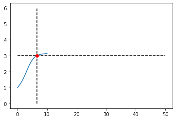
t0 = brentq(lambda y: y_interp(y)-3, 0, 10)
t0
#output: 6.562862752442042
plt.plot(t,y)
plt.plot([t0,t0],[0,6],'k--')
plt.plot([0,50],[3,3],'k--')
plt.plot(t0,3,'ro');

mark · August 2020

@Wiggenout You should indent anything that you want to appear as a code block four spaces. Have a look at this post and the references therein.

Sign in info

Quick Links

Categories

Numerically solve an IVP

Comments

Import necessary libraries: