A gentle introduction to maximum likelihood
Our objective here is to understand the basics of maximum likelihood estimation as applied to predictive sports analytics, like Kaggle's March Madness competition. While the code we develop here doesn't score particularly high there, we'll also discuss various improvements that could be made.
A very simple example
We'll start with a very simple example - one which is intuitive enough for us to "know" the answer right away but which also suggests the computational solution that we'll ultimately apply to more difficult situations - the so-called maximum likelihood method.
Example: I have a weighted coin that comes up heads with probability $p$ and comes up tails with probability $1-p$. Suppose I flip the coin 100 times and it comes up heads 62 times. What is your best guess for the the value of $p$?
I suppose that the obvious answer is $p\approx0.62$. Here's a computational approach that yields that exact value: First, the probability that we get 62 heads in 100 flips is
$$ f(p) = \binom{100}{62} \, p^{62}(1-p)^{38}. $$
The idea is to choose $p$ so that the probability of the observed event is maximized. Equivalently, since the logarithm is increasing, the maximum of $\log(f(p))$ occurs at the same place value of $p$. Thus, we might try to maximize $\log(f(p))$, which frequently has a simpler form. Putting this all together,
$$\begin{align} \frac{d}{dp} (\log(f(p))) &= \frac{d}{dp} \left( \log \binom{100}{62} + 62\,\log(p) + 38\, \log(1-p)\right) \\ &= \frac{62}{p} - \frac{38}{1-p} = \frac{100 p-62}{(p-1) p}. \end{align}$$
This last expression is zero precisely when $p=0.62$; thus, this is the choice of $p$ that maximizes the probability that our observed data could actually happen.
Exercise: Suppose that we flip a weighted coin $n$ times and $k$ heads result. Show that the maximum likelihood estimate of the probability $p$ that the coin produced heads is $k/n$.
A simple example
Let's suppose that three competitors or teams (numbered zero, one, and two) compete against each other twice each in some type of contest - football, basketball, tiddly winks, what have you. How might we rank them based on the results that we see? For concreteness, suppose the results are the following:
- Team zero beat team one twice and team two once,
- Team one beat team two once,
- Team two beat team zero and team one once each.
We might represent this diagrammatically as follows:
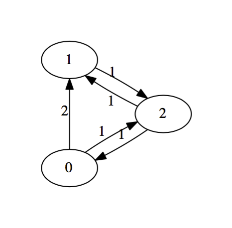
This configuration is called a directed graph or digraph. We construct it by placing an edge from team $i$ to team $j$ and labeling that edge with the number of times that team $i$ beat team $j$. We suppress zero edges. There an obvious matrix associated with a digraph called the adjacency matrix. The rows and column will be indexed by the teams. In row $i$ and column $j$, we place the label on the edge from team $i$ to team $j$. The adjacency matrix for this digraph is
$$M = \left(\begin{matrix} 0 & 2 & 1 \\ 0 & 0 & 1 \\ 1 & 1 & 0 \end{matrix}\right)$$
It seems reasonably clear that team zero should be ranked the highest, having beaten both competitors a total of 3 times out of 4 possible tries. Team one, on the other hand won only 1 game out of it's four tries, while team two seems to be in the middle, having split it's game with both competitors. Certainly, the teams listed from worst to first should be: $1$, $2$, $0$.
Let's try to re-derive this result using a maximum likelihood estimate. We suppose first that there is some vector $\vec{r} = \langle r_0, r_1, r_2 \rangle$ indicating the relative ratings of these teams. Ideally, if $p_{ij}$ denotes the probability that team $i$ beats team $j$, we might hope that $$ p_{ij} = \frac{r_i}{r_i+r_j}. $$ We'll use maximum likelihood to estimate such a vector. If $f(\vec{r})$ represents probability associated with a particular vector, I guess we have
$$ f(r_0,r_1,r_2) = \left(\frac{r_0}{r_0+r_1}\right)^2 \left(\frac{r_0}{r_0+r_2}\right) \left(\frac{r_2}{r_0+r_2}\right) \left(\frac{r_1}{r_1+r_2}\right) \left(\frac{r_2}{r_1+r_2}\right). $$
Thus,
$$ \log(f(r_0,r_1,r_2)) = 3\log(r_0) + \log(r_1) + 2\log(r_2) - 2\log(r_0+r_1) - 2 \log(r_0+r_2) - 2\log(r_1+r_2) $$
so we must find the value of $\vec{r}$ that maximizes this function. This boils down to solving the following system for $r_0$, $r_1$, and $r_2$.
$$\begin{align} \frac{d}{dr_0}\log(f(r_0,r_1,r_2)) &= \frac{3}{r_0} - \frac{2}{r_0+r_1} - \frac{2}{r_0+r_2} = 0 \\ \frac{d}{dr_1}\log(f(r_0,r_1,r_2)) &= \frac{1}{r_1} - \frac{2}{r_0+r_1} - \frac{2}{r_1+r_2} = 0 \\ \frac{d}{dr_2}\log(f(r_0,r_1,r_2)) &= \frac{2}{r_2} - \frac{2}{r_0+r_2} - \frac{2}{r_1+r_2} = 0. \end{align}$$
Note that the coefficients we see in these formulae can be read off of the adjacency matrix $M$. The 3, 1, and 2 in the expressions $3/r_0$, $1/r_1$, and $2/r_2$ are the row sums of $M$. The 2s in the expressions $2/(\log(r_i+r_j))$ arise from the sum $m_{ij}+m_{ji}$. These observations make it easier to write code to solve the equations when we have a larger matrix. The formula for the derivative of the log likelihood with respect to $r_i$ is
$$ \frac{d}{dr_i}\log(f(\vec{r})) = \frac{1}{r_i}\sum_{j=1}^n m_{ij} - \sum_{j=1}^n \frac{m_{ij}+m_{ji}}{r_i+r_j}. $$
Here's how we can solve this simpler system with Python:
from scipy.optimize import root
def g(r):
    r0=r[0]
    r1=r[1]
    r2=r[2]
    return [
        3/r0 - 2/(r0+r1) - 2/(r0+r2),
        1/r1 - 2/(r0+r1) - 2/(r1+r2),
        2/r2 - 2/(r0+r2) - 2/(r1+r2),
    ]
solution = root(g, [1/3,1/3,1/3])
if solution.success:
    r = solution.x/sum(solution.x)
    print(r)
else:
    print('uh-oh!')
Team zero is indeed the strongest team and team one the weakest. Furthermore, the model predicts that team zero will beat team one with probability $$ \frac{0.59181073}{0.59181073+0.13039543} \approx 0.819448466. $$
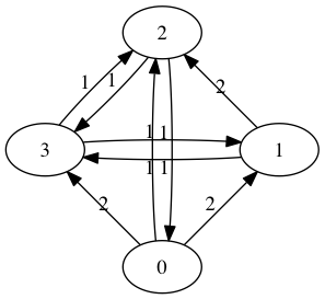
Exercise: Four teams play each other twice each; the results are shown in the directed graph below.
- Express the directed graph as an adjacency matrix.
- Write down the system of equations that you must solve to perform maximum likelihood method.
- Use Python to solve the system.
- What, according to the model, is the probability that team 2 beats team 3?
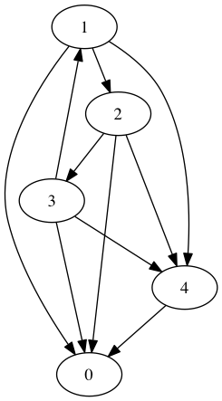
Exercise: Winless teams mess up the algorithm. Of course, we've got a pretty good clue how to rank them anyway so it might make sense to just remove them entirely. This might produce another winless team that might also need to be removed, and so on until the problem disappears. Taking this into account, perform a maximum likelihood estimate for the following digraph of games:
An actual example
Let's try this with some real data. First, let's import all the tools we'll need:
import pandas as pd
import numpy as np
from scipy.optimize import root
from scipy.sparse import dok_matrix
I've got a CVS file on my webspace that contains the results for all D1 games played in the 2018 college football regular season. This does not include conference championships or bowl games. I generated it by merging and simplifying the data available from Massey's ratings. Let's read it in and take a look:
cfb2018_df = pd.read_csv('https://www.marksmath.org/data/CFB_D1Results_2018.csv')
cfb2018_df.tail(7)
Turns out that that 130 different schools played 717 games. Let's simplify things by focusing on just one conference. Here's the Big Ten, with the exception of Rutgers, which was winless in the Big 10:
big10_results = cfb2018_df[ \
    ((cfb2018_df['team1_conference'] == 'B10') & \
    (cfb2018_df['team2_conference'] == 'B10')) & \
    ((cfb2018_df['team1_name'] != 'Rutgers') & \
    (cfb2018_df['team2_name'] != 'Rutgers'))
]
big10_schools = list(set(big10_results.team1_name.values).union(set(big10_results.team2_name.values)))
big10_schools.sort()
print(big10_schools)
Here is the matrix describing the wins:
n = len(big10_schools)
M = dok_matrix((n,n))
for i,game in big10_results.iterrows():
    if game.team1_score > game.team2_score:
        win_index = big10_schools.index(game.team1_name)
        lose_index = big10_schools.index(game.team2_name)
        M[win_index,lose_index] = 1
    elif game.team1_score < game.team2_score:
        win_index = big10_schools.index(game.team2_name)
        lose_index = big10_schools.index(game.team1_name)
        M[win_index,lose_index] = 1
M.todense().astype(int)
As is often the case for a matrix of moderate size, it's a bit easier to visualize as an adjacency graph.
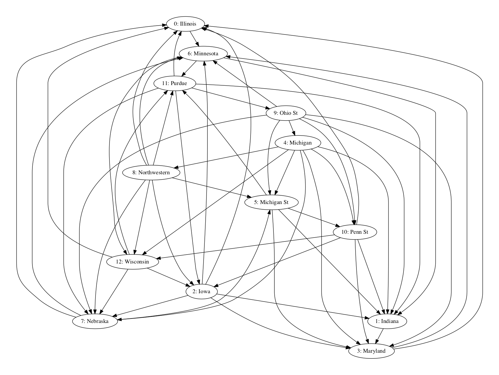
The following code uses that matrix to set up and solve the equations we need to find the maximum likelihood estimate.
def f(r):
    tot = sum(r)
    rr = [x/tot for x in r]
    eqs = [
        M[i].sum()/rr[i] - sum([(M[j,i]+M[i,j])/(rr[i]+rr[j]) for j in range(i)]) \
        for i in range(n)
    ]
    return eqs
sol = root(f,np.ones(n), method='lm')
print(sol.success)
sol.x
Here are the teams listed in order of strength, according to the algorithm:
sorted_indices = sol.x.argsort()
ranked = [(big10_schools[i], sol.x[i]) for i in sorted_indices]
ranked.reverse()
ranked
Well, that's disappointing - it looks like the model predicts that Ohio State will lose the Big Ten Championship game! It's close, though, as the prediction is barely above 50/50:
1.1574074364026428/(1.1574074364026428+1.1125025544257396)
Exercise: Perform a maximum likelihood ranking of the SEC. Note that Arkansas was winless and Mississippi was nearly winless, as they beat only Arkansas. You'll need to take that into account when constructing your matrix.