d = [2.57,4.43,2.09,7.68,4.77,2.12,5.13,5.71,5.33,3.31,7.49,4.91,2.58,1.08,6.60,3.91,3.97,6.18,5.90]
While it might be important for researchers to assess the threat of mercury in the ocean, they do not want to go kill more dolphins to get that data. What can they conclude from this data set, even though it's a bit too small to use a normal distribution?
The basics
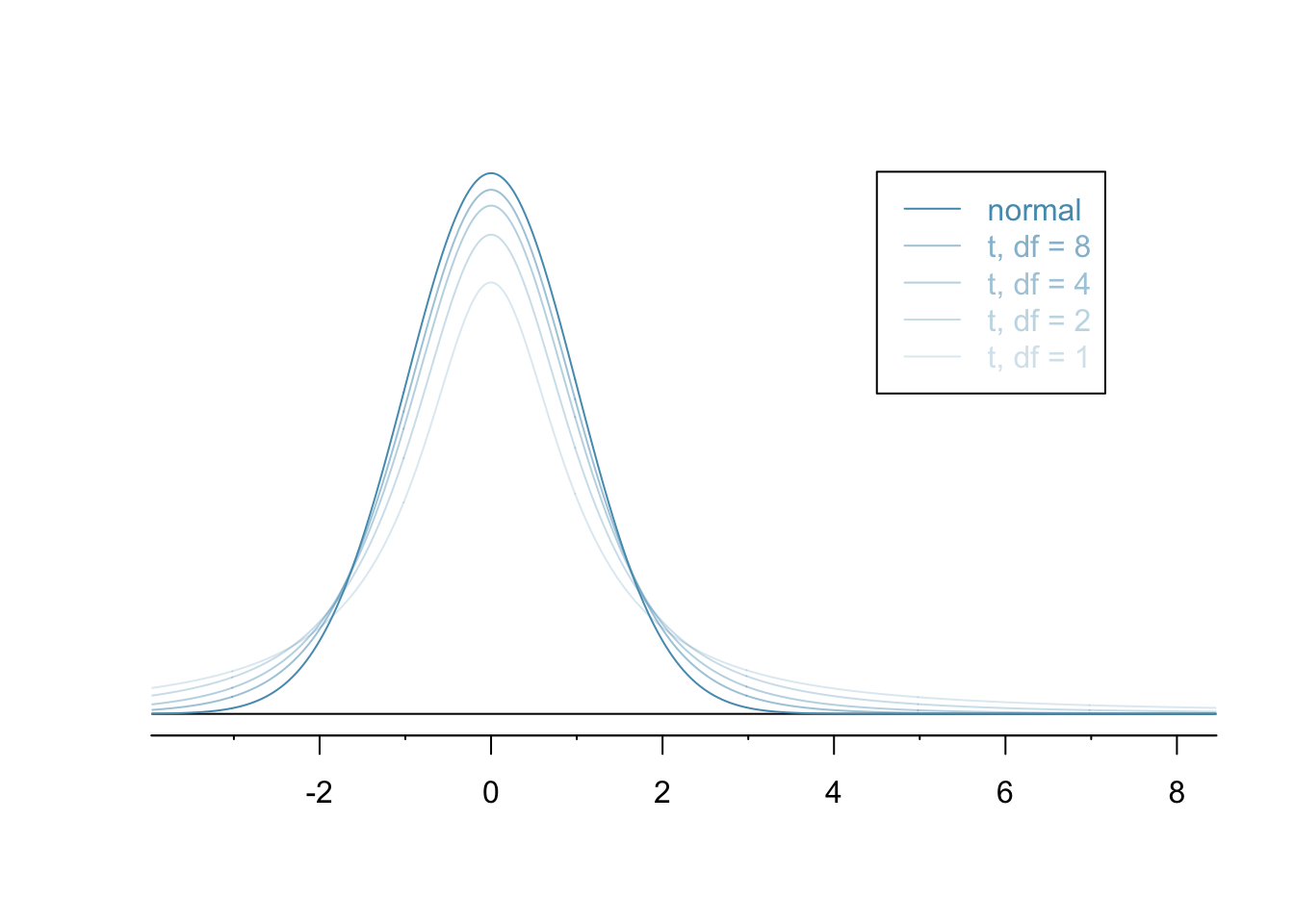
The normal distribution, as awesome as it is, requires that we work with large sample sizes.
The $t$-distribution is similar but better suited to small sample sizes.
Just as with the normal distribution, there's not just one $t$-distribution but, rather, a family of distributions.
Just as there's a formula for the normal distribution, there's a formula for the $t$-distribution. It's a bit more complicated, though: $$ f(t) = \frac{\left(\frac{\nu-1}{2}\right)!} {\sqrt{\nu\pi}\,\left(\frac{\nu-2}{2}\right)!} \left(1+\frac{t^2}{\nu} \right)^{\!-\frac{\nu+1}{2}} $$ The parameter $\nu$ is an integer representing the degrees of freedom which is the sample size minus one.
Like all continuous distributions, we compute probabilities with the $t$-distribution by computing the area under a curve. We do so using either a computer or a table.
The mean of the $t$-distribution is zero and its variance is related to the degrees of freedom $\nu$ by $$\sigma^2 = \frac{\nu}{\nu-2}.$$
Unlike the normal distribution, there's no easy way to translate from a $t$-distribution with one standard deviation to another standard one. As a result, it's less common to use tables and more common to use software than it is with the normal.
Given a particular number of degrees of freedom, however, there is a standard way to derive a $t$-score that's analogous to the $z$-score for the normal distribution. This $t$-score is a crucial thing that you need to know when using tables for the $t$-distribution.
Finding the confidence interval
Finding a confidence interval using a $t$-distribution is a lot like finding one using the normal. It'll have the form $$ [\overline{x}-ME, \overline{x}+ME], $$ where the margin of error $ME$ is $$ ME = t^* \frac{\sigma}{\sqrt{n}}. $$
Of course, we can compute the mean and standard deviation using NumPy:
import numpy as np
m = np.mean(d)
s = np.std(d, ddof=1)
[m,s]
The crazy looking ddof parameter forces np.std to compute the sample standard deviation, rather than the population standard deviation - i.e. it uses an $n-1$ in the denominator, rather than an $n$.
Next, the multiplier $t^*$ can be computed using t.ppf from the scipy.stats module:
from scipy.stats import t
tt = t.ppf(0.975,df=18)
tt
Thus, our confidence interval is:
[m-tt*s/np.sqrt(19), m+tt*s/np.sqrt(19)]
Using a table
Note that we can also find that $t^*=2.1$ in the $t$-table on our webpage, where we see something that looks like so:
| one tail | 0.100 | 0.050 | 0.025 | 0.010 | 0.005 |
| two tails | 0.200 | 0.100 | 0.050 | 0.020 | 0.010 |
| df 1 | 3.08 | 6.31 | 12.71 | 31.82 | 63.66 |
| 2 | 1.89 | 2.92 | 4.30 | 6.96 | 9.92 |
| ... | ... | ... | ... | ... | ... |
| 18 | 1.33 | 1.73 | 2.10 | 2.55 | 2.88 |
The entries in this table are called critical $t^*$ values. The columns indicate several common choices for confidence level and are alternately labeled either one-sided or two. The rows correspond to degrees of freedom. Now, look in the row where $df=18$ and where the two-sided test is equal to 0.05. we see that $t^*=2.1$.
Chips Ahoy!
In 1998, Nabisco announced its 1000 chip challenge, claiming that every bag of Chips Ahoy cookies contained at least 1000 chips. A group of students counted the chips in 16 bags of cookies and found the following data:
d = [1219,1214,1087,1200,1419,1121,1325,1345,1244,1258,1356,1132,1191,1270,1295,1135]
Create a $99\%$ confidence interval for the number of chips in the bag.