The normal distribution
Of all the distributions that you meet in an introductory statistics class, by far the most important is the normal distribution, which is defined by
$$f_{\mu,\sigma}(x) = \frac{1}{\sqrt{2\pi}\sigma} e^{-(x-\mu)^2/(2\sigma^2)}.$$
In the case where $\mu=0$ and $\sigma=1$, this simplifies a bit to
$$f_{0,1}(x) = \frac{1}{\sqrt{2\pi}} e^{-x^2/2}.$$
The graph of a normal distribution is the classic bell shaped curve. It's heaviest at it's mean $\mu$ and gets lighter as you move away from the mean. Here are the graphs of normal distributions for several choices of $\mu$ and $\sigma$:
%matplotlib inline
import matplotlib.pyplot as plt
import numpy as np
from matplotlib import rcParams
rcParams['figure.figsize'] = (9,6)

def f(x,m,s):
    return np.exp(-(x-m)**2/(2*s**2))/(np.sqrt(2*np.pi)*s)
xs = np.linspace(-5,6,200)
plt.plot(xs,f(xs,0,1), color='green')
plt.plot(xs,f(xs,-2,0.4), color='red')
plt.plot(xs,f(xs,2,2), color='blue')
plt.text(-0.3,.45,'$\mu=0$\n$\sigma=1$', color='green')
plt.text(-3.6,0.6,'$\mu=-2$\n$\sigma=0.2$', color='red')
plt.text(4,0.14,'$\mu=2$\n$\sigma=2$', color='blue');

You can play with these parameters dynamics with my normal distribution demo.
Importance
The normal distribution is important because it is often a good approximation to other distributions. For example, let's plot a binomial distribution along with the normal distribution that has the same mean and standard deviation.
from scipy.special import binom as binomial_coefficient

n = 20
p = 0.35
vals = [int(binomial_coefficient(n,k))*p**k*(1-p)**(n-k) for k in range(n+1)]
for i,v in enumerate(vals):
    plt.plot([i,i],[0,v], 'k', linewidth=0.4)
    plt.plot(i,v, 'ok')

m = n*p
s = np.sqrt(n*p*(1-p))
xs = np.linspace(-2,n+2,200)
plt.plot(xs,f(xs,m,s));

Now, the binomial distribution arises by running a number of trials and determining the proportion of successes. More generally, the normal distribution is a good approximation whenever an averaging process generates data.
It does not matter how the original data is distributed - the normal arises from the averaging process.
For example, here's a histogram of $10,000$ uniformly generated points:
from scipy.stats import uniform

a = 3
b = 7
u = uniform.rvs(a,b-a,10000)
plt.hist(u, bins = np.linspace(a,b,8), edgecolor='black', density=True);

Now, let's modify that a bit. Rather than generate a buch of points that are uniformly distributed, we'll generate a random point by
- First generating 100 uniformly distributed points and then
- Computing their average.
If we do this 10000 times, we get:
a = 3
b = 7
n = 100
au = [uniform.rvs(a,b-a,n).mean() for i in range(10000)]
plt.hist(au, bins = 20, edgecolor='black', density=True);
m = (a+b)/2
s = (b-a)/np.sqrt(12*n)
xs = np.linspace(m-3.5*s, m+3.5*s, 200)
plt.plot(xs,f(xs,m,s), 'k', linewidth=2);

Again, it's absolutely crucial to understand that neither a Bernouli distribution nor the uniform distribution are anything like a normal distribution. However, if we form a binomial distribution by adding a bunch of Bernoulis or we average out a bunch of uniform distributions, the result is well approximated by a normal. There's a theorem called the central limit theorem that explains why this must happen.
Working with normal distributions
The standard normal
Suppose we know that $X$ has a standard normal distribution. We can compute $P(a<X<b)$ just as we would any probability from a density function:
$$P(a<X<b) = \frac{1}{\sqrt{2\pi}} \int_a^b e^{-x^2/2} dx.$$
A key difference between the normal distribution and the examples that we've worked with before is that the PDF has no elementary antiderivative! As a result, we typically estimate this type of integral using numerical integration.
For example, if $X$ has a standard normal distribution, then the probability that $X$ lies in the interval $[0,1]$ is
$$P(0<X<1) = \frac{1}{\sqrt{2\pi}} \int_0^1 e^{-x^2/2} dx.$$
We can compute this in Python using scipy.integrate.quad:
from scipy.integrate import quad
quad(lambda x: f(x,0,1), 0,1)
The response is an (val,err) pair, where val is the estimate to the value the integral and err is a bound on the error associated with the estimate. In particular, the probability that a standard normally distributed random variable lies in the interval $[0,1]$ is about 0.34.
Other normal integrals
It turns out that any probability computation involving any normal distribution can be computed using an integral involving the standard normal. This can be shown using $u$-substitution.
Claim: $$\frac{1}{\sqrt{2\pi}\sigma} \int_a^b e^{-(x-\mu)^2}/(2\sigma^2) dx = \frac{1}{\sqrt{2\pi}} \int_{(a-\mu)/\sigma}^{(b-\mu)/\sigma} e^{-x^2/2} dx.$$ Justification: Let $u=(x-\mu)/\sigma$. Then, $du = (1/\sigma)dx$ and
$$ \begin{align} \frac{1}{\sqrt{2\pi}{\sigma}} \int_a^b e^{-(x-\mu)^2/(2\sigma^2)} dx &= \frac{1}{\sqrt{2\pi}} \int_a^b e^{-\frac{1}{2}\left(\frac{x-\mu}{\sigma}\right)^2} \, \frac{1}{\sigma}dx \\ &= \frac{1}{\sqrt{2\pi}} \int_{(a-\mu)/\sigma}^{(b-\mu)/\sigma} e^{-u^2/2} du = \frac{1}{\sqrt{2\pi}} \int_{(a-\mu)/\sigma}^{(b-\mu)/\sigma} e^{-x^2/2} dx. \end{align} $$
Comment: In terms of probability comutations, this can be rephrased as follows: If $X$ is normally distributed with mean $\mu$ and standard deviarion $\sigma$, then $Z=(X-\mu)/\sigma$ is a standard normal and
$$P(a<X<b) = P\left(\frac{a-\mu}{\sigma}<Z<\frac{b-\mu}{\sigma}\right).$$
This computation $Z=(X-\mu)/\sigma$ is sometimes called a $Z$-score and is the fundamental tool that converts any normal random variable to a standard normal.
Example: Suppose that $X$ is normally distributed with a mean of 50 and a standard deviation of 10. What is the probability that $X$ lies between 50 and 60?
Solution: We comute the $Z$-scores of the endpoints to get
$$P(50<X<60) = P((50-50)/10 < Z < (60-50)/10) = P(0<Z<1).$$
This is the exact computaton that we did before so we know the result is about $0.34$.
Rules of thumb for the normal
Some common rules of thumb for the normal distribution state that
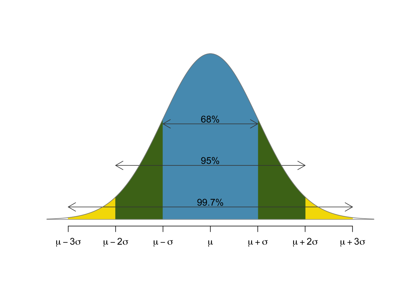
- 68% of the population lies within one standard deviation of the mean,
- 95% of the population lies within two standard deviations of the mean, and
- 99.7% of the population lies within three standard deviations of the mean.
This can be illustrated with a normal curve as follows:
The specific numbers come from computations involving the standard normal. The fact that we can use just the standard normal and extend the result to any normal arises from the $Z$-score:
$$P(\mu-n\sigma < X < \mu+n\sigma) = P\left(\frac{(\mu-n\sigma)-\mu}{\sigma} < Z < \frac{(\mu+n\sigma)-\mu}{\sigma}\right) = P(-n < Z < n).$$
Example: SAT are designed to be normally distributed with a mean of 500 and a standard deviation of 100. If you score a 700, at what percentile do you lie?
Solution: The rules of thumb make this easy! 700 lies two standard deviations past the mean. Since 95% of the scores are within 2 standard deviation, 5% are more than 2 standard deviations from the mean. Half of that 5% lies above 700 and half of that 5% lies below 300. Thus 2.5% lie above 700 putting that score at the $97.5^{\text{th}}$ percentile.
Working with software
The scipy.stats module has a number of functions for working directly with probability distributions such as the binomial and the normal. Let's import a couple.
from scipy.stats import binom, norm
These are objects which bundle important methods for working their respective type of distributions. For example, norm contains norm.pdf for the probability density function and norm.cdf for working with the cummulative density function. The relationship is as follows:
xs = np.linspace(-4,4,200)
ax = plt.subplot(2,1,1)
xs2 = np.linspace(-4,-1,50)
plt.plot(xs,norm.pdf(xs))
plt.plot([-1,-1],[0,norm.pdf(-1)],'k--')
plt.text(-3,0.2, 'area = 0.1586')
plt.title('PDF')
ax.fill_between(xs2,0,norm.pdf(xs2))
ax = plt.subplot(2,1,2)
plt.plot(xs,norm.cdf(xs))
plt.plot(-1,norm.cdf(-1), 'ok')
plt.text(-2.5,0.2, 'value = 0.1586')
plt.title('CDF');

Thus, the CDF tells us how much area has accumulated under the PDF up to that point. The 0.1586 above comes from the following computaion:
norm.cdf(-1)
In terms of a probability computation, this means that if $X$ has a standard normal distribution, then
$$P(X<-1) \approx 0.1586.$$
An example
Suppose I have an unfair coin that comes up heads 1/3 of the time. If I flip the coin 1000 times, what is the probability that I get at most 300 heads?
The most direct approach to answer this question is to use the binom.cdf method:
binom.cdf(300,1000,1/3)
Note that there are three inputs to binom.cdf(x,n,p):
x- the cuttoffn- the number of trialsp- the probability of success
An alternative is to approximate with norm.cdf:
norm.cdf(300.5,1000/3,np.sqrt(1000*2/9))
Again, there are three inputs to norm.cdf(x,m,s):
x- the cuttoffm- the means- the standard deviation
The mean and standard deviation are chosen to agree with the mean and standard deviation of the corresponding binomial. The 300.5, rather than 300, arises from the so-called continutity correction and accounts for the fact that we are approximating a discrete distribution with a continuous one.
Working with tables
Classically, the way to compute probabilities associated with a normal distribution is to read from a table.
For example, suppose that $Z$ is standard normally distributed and I want to compute $P(Z<0.53)$ I can just read the value of 0.7019 right off of this table:
| Z | 0.00 | 0.01 | 0.02 | 0.03 | 0.04 |
|---|---|---|---|---|---|
| ... | ... | ... | ... | ... | ... |
| 0.5 | 0.6915 | 0.6950 | 0.685 | 0.7019 | 0.7054 |
| ... | ... | ... | ... | ... | ... |
If I wanted to know $P(0<Z<0.53)$, I could compute $$P(0<Z<0.53) = P(Z<0.53) - P(Z<0) = 0.7019 - 0.5 = 0.2019.$$
If I have a normally distributed random variable that is not necessarily a standard normal, I can just translate it to a standard normal by comuting $Z$-scores.