The binomial distribution
The binomial distribution is a discrete distribution that plays a special role in statistics for many reasons. The general idea is as follows: Suppose that a single experiment has probability of success $p$ and probability of failure $1-p$. We turn this into random variable by assigning numeric values, say success yields a $1$ and failure yields a $0$. We then run the experiment a number of times, say $n$, and count the number of successes. This yields an integer between $0$ and $n$ inclusive. The binomial distribution tells us the probability of each of those $n+1$ outcomes.
Flipping a fair coin
Suppose our experiment is just flipping a coin, that a head represents success, and that a tail represents failure. Thus, with one flip, we can get a $0$ or a $1$ with equal probability $1/2$ each.
Now suppose we flip a coin 5 times and count how many heads we get. This will generate a random number $X$ between 0 and 5 but they are not all equally likely. The probabilities are:
- $P(X=0)=1/32$
- $P(X=1)=5/32$
- $P(X=2)=10/32$
- $P(X=3)=10/32$
- $P(X=4)=5/32$
- $P(X=5)=1/32$
Note that the probability of getting any particular sequence of 5 heads and tails is $$\frac{1}{2^5} = \frac{1}{32}.$$ That explains the denominator of 32 in the list of probabilities. The numerator is the number of ways to get that value for the sum. Note that these are exactly the binomial coefficients!
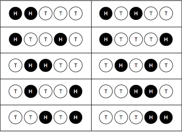
For example, there are 10 ways to get 2 heads in 5 flips:

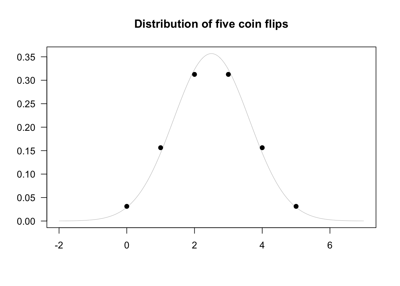
If we plot the possible outcomes vs their probabilities, we get something like the following:

The curve that we see is the normal curve with the same mean and standard deviation. As we'll learn soon, this curve can be used to model the binomial distribution, as well as many other distributions. The relationship becomes more pronounced as we increase the flip count:

Some code
I have an unfair coin that comes up heads $2/3$ of the time. If I flip the coin 100 times, what is the probability that I get at most 60 heads?
Using a binomial distribution, its easy to answer this in principal. We can write the solution as a sum:
$$\sum_{k=0}^{60} \begin{pmatrix}60\\k\end{pmatrix} \left(\frac{2}{3}\right)^k \left(\frac{1}{3}\right)^{60-k}.$$
Here's a good decimal approximation to this with Python:
from scipy.special import binom
n = 100
p = 2/3
sum([binom(n,k)*p**k*(1-p)**(n-k) for k in range(61)])
The scipy.stats module has tools to work directly with distributions like the binomial and the normal. For example, here's how to use the binom.cdf function (for binomial Cummulative Distribution Function or CDF) to perform the same computation:
from scipy.stats import binom, norm
binom.cdf(60,100,2/3)
We'll learn very soon how to use the normal distribution to obtain a good estimate to this computation.
from scipy.stats import norm
from numpy import sqrt
norm.cdf(60.5, 200/3, sqrt(100*p*(1-p)))