Bifurcation diagrams

A bifurcation diagram is yet another geometric tool to help us understand the emergence of chaos in the logistic family - as well as in other parametrized families of functions. It is one of the iconic images of chaos.

Explanation

Recall the logistic function: \[f_r(x) = rx(1-x).\] The symbol \(r\) is called a parameter. As we've learned, the long term, iterative behavior of the logistic function is very dependent on the parameter. When \(r\) is small (smaller than \(3\), in fact), the iterates of \(f_r\) converge to a single fixed point. Once \(r\) is larger than 3, the behavior is more complicated.

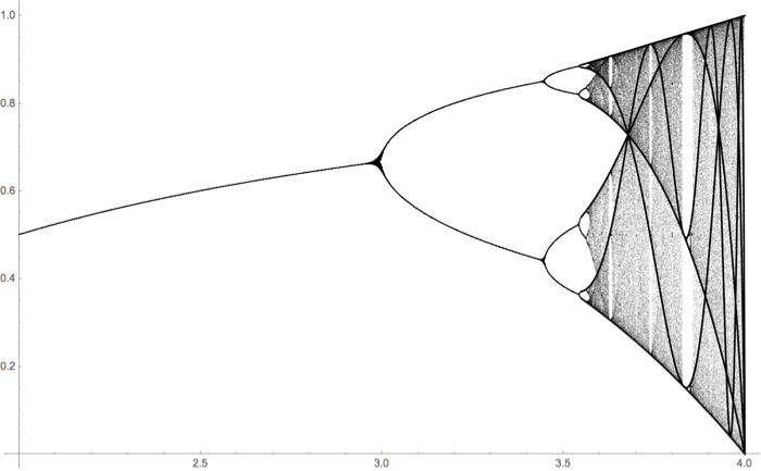
In order to understand the complications, we generate the bifurcation diagram as follows: Given \(r\) in a certain range, perhaps \(2\leq r \leq 4\), we iterate the corresponding logistic function \(f_r(x)=rx(1-x)\) starting from the point \(x=1/2\) where the maximum occurs. We iterate a lot - like \(1,000\) times. We discard the first hundred or so iterates because we don't care about transient behavior. We then plot the remaining points \((r,y)\). These points lie in a vertical column with contant horizontal value \(r\).

Hopefully, this annotated bifurcation diagram helps illustrate this all a bit more clearly:

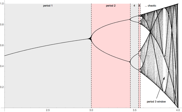
We can see that as \(r\) increases, the two cycle bifurcates into a four cycle at around \(r\approx3.45\). That happens again and again and again as we go through a so called period doubling cascade. That infinite cascade actually completes around \(r\approx3.57\) and chaos ensues afterward. There are, however, windows of periodic calm interspersed; the most prominent being the period 3 window around \(r\approx 3.832\)