Modeling a central orbit
Suppose that a single object $\mathbf{p}$ revolves around a much, much larger object moving under the gravitational influence of the larger body. We can model the motion of $\mathbf{p}$ in a coordinate system with the larger object at the origin. There will be a single force acting on $\mathbf{p}$ directed toward the origin and whose magnitude is proportional to the reciprocal of the distance from $\mathbf{p}$ to the origin squared. If $\vec{p}(t)$ is the vector position of $\mathbf{p}$ at time $t$, then the force $F$ is
$$F = -g\frac{\vec{p}(t)}{\left\|\vec{p}(t)\right\|^3},$$where $g$ is a positive proportionality constant. The negative sign ensures that the force is directed back towards the origin. By Newton's second law $F=m\vec{a}$, this induces an acceleration of $\mathbf{p}$. Absorbing the mass into the proportionality constant, we find that $\vec{p}(t)$ obeys the second order differential equation
$$\vec{p}''(t) = -G\frac{\vec{p}(t)}{\left\|\vec{p}(t)\right\|^3}.$$This is the basic vector equation describing motion through a gravitational field. If we want the joy of visualization, we might assume the motion is restricted to a plane and write $\vec{p}(t) = \langle x(t),y(t) \rangle$. The vector equation may then be written as the system
$$ \begin{align} x''(t) &= -G \frac{x(t)}{(x(t)^2 + y(t)^2)^{3/2}} \\ y''(t) &= -G \frac{y(t)}{(x(t)^2 + y(t)^2)^{3/2}}. \end{align} $$Given a specific value of $G$ with an initial position and velocity, this system may be solved in closed form. To do so with SciPy, we need to write it as a first order sytem by introducing variables $v_x = x'$ and $v_y = y'$. The system is then
$$ \begin{align} x'(t) &= v_x(t) \\ y'(t) &= v_y(t) \\ v_x'(t) &= -G \frac{x(t)}{(x(t)^2 + y(t)^2)^{3/2}} \\ v_y'(t) &= -G \frac{y(t)}{(x(t)^2 + y(t)^2)^{3/2}}. \end{align} $$To solve this in SciPy, we need to write this as a single vector equation $s' = F(s)$ by introducing the vector $$\vec{s} = \langle s_0, s_1, s_2, s_3 \rangle = \langle x, y, v_x, v_y \rangle$$ and the function $$F\left(\vec{s}\right) = \langle s_2, s_3, -G s_0/(s_0^2 + s_1^2), -G s_1/(s_0^2 + s_1^2) \rangle.$$
Let's solve the system obtained by placing the $\mathbf{p}$ one unit to the right of the origin moving up with a speed of one unit per time click. Symbolically: $$ \begin{align} x(0) &= 1 \\ y(0) &= 0 \\ v_x(0) &= 0 \\ v_y(0) &= 1. \end{align} $$
Let's also suppose that $G=3$.
# Imports
# SciPy's numerical ODE solver
from scipy.integrate import odeint
# The fabulous numpy library:
import numpy as np

# Parameters
G = 3
x0 = 1
y0 = 0
vx0 = 0
vy0 = 1

# In the following definition of F, s is a state vector whose components represent the following:
#   s[0]: Horizontal or x position
#   s[1]: Vertical or y position
#   s[2]: Horizontal velocity
#   s[3]: Vertical velocity
# In general, F can depend upon time t as well. Although our F is independent of t, we still need to
# indicate that it is a possible variable.

def F(s,t): return [s[2],s[3],
    -G*s[0]/(s[0]**2 + s[1]**2)**(3/2),
    -G*s[1]/(s[0]**2 + s[1]**2)**(3/2),
]

# We'll solve the system for the following values of t, namely
# 100 equally spaced values between 0 and 2.
t = np.linspace(0,2,50)

# Solve it!
solution = odeint(F,[x0,y0,vx0,vy0],t)
So, what'd we do? Well, solution should be a list of 50 items; each of those should be an $\langle s_0,s_1,s_2,s_3 \rangle$ quadruple indicating the $x$-position, $y$-position, $x$-velocity, and $y$-velocity at the corresponding $t$ value. Let's look at the first 10 of them:
solution[:10]
Not super informative. Perhaps a plot would help? Here are the locations of the object at the times indicated by t.
%matplotlib inline
import matplotlib.pyplot as plt
x = solution[:,0]
y = solution[:,1]
plt.plot(x,y, '.');

Looks interesting! As expected, we get an ellipse. The weird spacing arises from the varying speed of $\mathbf{p}$, which moves faster the closer it is to the origin. We can also sorta see that we've started to traverse the ellipse a second time, but just a bit. We can find the period fairly precisely by interpolating these points to obtain a spline function $f$ and then finding a root of the second coordinate of $f$ between 1 and 2.
from scipy.interpolate import interp1d
from scipy.optimize import brentq
y = solution[:,1]
f = interp1d(t, y)
period = brentq(f,1,2)
period
Looks good! Now, let's compute a higher resolution solution over one period.
t = np.linspace(0,period,1001)
solution = odeint(F,[x0,y0,vx0,vy0],t)
x = solution[:,0]
y = solution[:,1]
plt.plot(x,y)

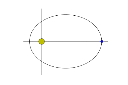
We can go overboard and write a function that generates a picture that illustrates where the object is in relation to its sun.
def pic(n=0):
    plt.plot(x,y, 'k')
    plt.plot(x[n],y[n], 'o', markersize=8)
    ax = plt.gca()
    ax.set_xlim([-0.3,1.1])
    ax.set_ylim([-0.55, 0.55])
    ax.set_xticks([])
    ax.set_yticks([])
    ax.set_aspect(1)
    ax.spines['left'].set_position('zero')
    ax.spines['left'].set_zorder(0)
    ax.spines['left'].set_alpha(0.4)
    ax.spines['right'].set_color('none')
    ax.spines['bottom'].set_position('zero')
    ax.spines['bottom'].set_zorder(0)
    ax.spines['bottom'].set_alpha(0.4)
    ax.spines['top'].set_color('none')
    plt.plot(0,0, 'yo', markersize=20)
    sp = ax.spines['left']
    sp.set_zorder(0)
pic(123)

This makes it easy to generate visualizations. If you're viewing this live, you can interact with it as follows:
from ipywidgets import interact
interact(pic, n=(0,1000,1));

The frames of the animation at the top of the page were generated as follows:
for i in range(0,1000,20):
    if(i<10):
        file_name = "pic00"+str(i)+".png"
    elif(10<=i<100):
        file_name = "pic0"+str(i)+".png"
    else:
        file_name = "pic"+str(i)+".png"
    pic(i);
    fp = open(file_name,'w')
    plt.savefig(file_name)
    fp.close()
    plt.close()
Again, this generates the individual frames. A single animated GIF (like the one at the top of the page) can be generated via an external program like ImageMagick. Once you've got that installed, the animated gif is created via the system command
convert -delay 1 *.png -loop 0 anim.gif
The main reason I actually went through all this was to generate output for a javascript visualization. That program reads JSON generated by the following:
import json
to_export = []
cnt = 0
for x in np.delete(solution, -1, 0):
    to_export.append({"t": t[cnt], "x":x[0], "y":x[1], "speed":np.sqrt(x[2]**2+x[3]**2)})
    cnt=cnt+1
file_handle = open('orbit.json','w')
json.dump(to_export,file_handle, indent=1)
file_handle.close()